one year of data that includes 11 measurements at one minute intervals for 21 sub-meters. AMPds also includes natural gas and water consumption data. Finally ...
Accepted at The Annual Electrical Power and Energy Conference (EPEC 2013).
AMPds: A Public Dataset for Load Disaggregation and Eco-Feedback Research Stephen Makonin∗† , Fred Popowich∗ , Lyn Bartram‡ Bob Gill§ , Ivan V. Baji´c¶ ∗ Computing
Science, ¶ Engineering Science, ‡ Interactive Arts + Technology, Simon Fraser University Centre, § School of Energy, British Columbia Institute of Technology Email: {smakonin, popowich, lyn, ibajic}@sfu.ca, {Stephen Makonin, Bob Gill}@bcit.ca † Technology
Abstract—A home-based intelligent energy conservation system needs to know what appliances (or loads) are being used in the home and when they are being used in order to provide intelligent feedback or to make intelligent decisions. This analysis task is known as load disaggregation or non-intrusive load monitoring (NILM). The datasets used for NILM research generally contain real power readings, with the data often being too coarse for more sophisticated analysis algorithms, and often covering too short a time period. We present the Almanac of Minutely Power dataset (AMPds) for load disaggregation research; it contains one year of data that includes 11 measurements at one minute intervals for 21 sub-meters. AMPds also includes natural gas and water consumption data. Finally, we use AMPds to present findings from our own load disaggregation algorithm to show that current, rather than real power, is a more effective measure for NILM. Index Terms—Power Meter, Current, Dataset, Load Disaggregation, Eco-Feedback, Single-Measurement, Maximum a Posteriori (MAP), Energy Conservation
I. I NTRODUCTION Currently, much of the world is focused on reducing electricity consumption; our increase in consumption is neither economically nor environmentally sustainable. Additionally, there is a growing consensus that environmental and economical sustainability are inextricably linked. As the cost of power rises, we must find technological solutions that help reduce and optimize energy use. For homeowners and occupants, one way to achieve this goal is to monitor their power consumption by understanding appliance usage through an effective ecofeedback device or display mechanism. When designing and implementing an intelligent energy conservation system for the home, it is essential to have insight into the activities and actions of the occupants. In particular, it is important to understand what appliances are being used and when. In the computational sustainability research community this is known as load disaggregation or nonintrusive load monitoring (NILM) (Section II). Currently there are a handful of datasets that load disaggregation researchers can use (Section II-A). Each dataset has its own limitations– mostly these datasets capture short-term power usage and only provide readings of real power. We introduce the Almanac of Minutely Power dataset (AMPds) containing one year of data that includes 11 measurements at one minute intervals for 21 sub-meters. Furthermore, data for natural gas and water consumption are provided (Section III). Additional measurements are included to support the argument that current (not real
power) may be a better measurement for load disaggregation (Section IV). Using AMPds, we present our initial findings of a load disaggregation algorithm that uses single-measurement MAP (Maximum a Posteriori) criteria (Section V). Finally, we discuss how AMPds is being used to develop and test the usability of eco-feedback devices (Section VI). II. L OAD D ISAGGREGATION In the computational sustainability research field, load disaggregation goes by many names and acronyms, including non-intrusive load monitoring (NILM) and nonintrusive appliance load monitoring (NIALM or NALM). Early research by Sultanem [1] and then Hart [2] proposed strategies to disaggregate loads using whole-house power readings. Recently researchers have focused on using smart meter data as a more realistic solution [3]–[9]. However, we question whether using real power to disaggregate is the best choice of measurement (see Section IV for details). We have previously identified five key problems which further challenge the success of a load disaggregation system [10]: multiple, simultaneous load events, noisy power signals, dynamic and changing usage, computational cost and complexity, and privacy. Of those five, dynamic and changing usage is one of the motivations for AMPds. Dynamic and changing usage means, that over a period of time, the number of appliances within a home can increase and decrease. They can also be replaced as in the case of an old dishwasher breaking down which is then replaced with new, more energy efficient model. These changes are coupled with the fact that occupant-home interaction varies greatly from one home to another, or over a long period of time [11]. So it can be difficult for a load disaggregation system to generalize over data from other homes or other periods of time. For this reason, load disaggregation algorithms that rely on contextaware and/or time-based/temporal modelling [12]–[14] needs to be tested for accuracy on datasets that capture long-term usage of appliances. There are different types of appliances that need to be considered by NILM algorithms. Hart identifies four different applicance types: simple on/off, finite-state, constantly on, and continuously variable [2]. Zeifman, for example, only considers simple on/off appliance disaggregation [8]. Many home appliances (including some LED lighting) have embedded electronics that allow for different running options
c 2013 IEEE. The original publication is available for download at ieeexplore.ieee.org. Copyright
and controls, resulting in a load that does not have a simple on/off behaviour. So the real challenge for load disaggregation algorithms is the need to detect complex, finite-state appliances and loads. Our preliminary load disaggregation algorithm handles all of Hart’s four appliance types. A. Other Datasets There are existing datasets for load disaggregation researchers to use–each with significant limitations. These datasets generally provide only a power measurement for the whole-house and/or multiple house loads. There are only a handful of datasets due to the costs involved with equipment purchase and installation. The MIT Reference Energy Disaggregation Data Set or REDD [15] supplies high and low frequency readings specifically for residential load disaggregation for a short period of time (from a few weeks to a few months). Zeifmann [8] found that whole-house measurements were provided in apparent power and individual circuits were measured in real power. Consequently, the sum of individual circuits did not equal the whole-house. The CMU Building-Level fUlly labeled Electricity Disaggregation dataset or BLUED [16] contains high frequency readings of a single family home with a list of appliance events, but only for one week. The UMASS Smart* Home Data Set [17] contains high and low frequency readings, but is not specifically designed for NILM evaluation. The Tracebase dataset [18] contains appliance power traces sampled at intervals of one second. There are organizations that provide datasets for their customers. For example, Green Button has a number of sample datasets publicly available from their website (http://www.greenbuttondata.org/greendevelop.aspx). The Plugwise dataset was used by [4] but is only available upon the submission of a request to the company. III. T HE AMP DS DATASET Our dataset is a record of energy consumption of a single house using 21 sub-meters for an entire year (from April 1, 2012 to March 31, 2013) at one minute read intervals. We chose a one minute interval due to concerns over data communication network saturation, but this comes at a cost of loss of fidelity (i.e. missing power measurement spikes that could help identify loads more easily) [6]. We monitored a house built in 1955 in the greater Vancouver region in British Columbia, which underwent major renovations in 2005 and 2006–receiving a Canadian Government EnerGuide rating of 82%. Using branch circuit power metering (BCPM, see Figure 1) we metered 21 breakers from the house power panel. Table IV lists the 21 sub-metered breakers/loads. The two BCMP units were queried once per minute by an industrial data acquisition server (see Figure 3(a)). Table I lists the BCPM measurements captured. For natural gas metering there were two meters: the wholehouse meter (WHG) and the gas furnace meter (FRG). For water metering there were also two meters: the whole-house meter (WHW) and the hot water meter (HTW). Figure 2 shows
Fig. 1. Two DENT PowerScout 18 units metering 24 loads at the electrical circuit breaker panel. Measurements are read over a RS-485/Modbus communication link by data acquisition equipment (see Figure 3(a)). TABLE I P OWER M EASUREMENTS C APTURED Column 0 1 2 3 4 5 6 7 8 9 10 11
Description
Units
Unix Timestamp (since Epoch) Voltage (V) Current (I) Frequency (f ) Displacement Power Factor (DPF) Apparent Power Factor (APF) Real Power (P) Real Energy (Pt) Reactive Power (Q) Reactive Energy (Qt) Apparent Power (S) Apparent Energy (St)
s V A Hz ratio ratio W Wh VAR VARh VA VAh
the pulse meters used. Table II and Table III lists the pulse measurements captured by the data acquisition server (see Figure 3(b)) for both natural gas and water consumption. TABLE II NATURAL G AS M EASUREMENTS C APTURED Column 0 1 2 3
Description
Units
Unix Timestamp (since Epoch) Pulse Counter Average Rate Instantaneous Rate
s dm3 dm3 /h dm3 /h
The data acquisition servers (Figure 3) push data captured to a remote, off-site MySQL server via HTTP POSTS. When creating the AMPds comma separated value (CSV) files, we first cleaned the dataset by removing incomplete captures (i.e.
TABLE III WATER M EASUREMENTS C APTURED Column 0 1 2 3
(a) Gas Main Meter
(b) Gas Furnace Meter
Description
Units
Unix Timestamp (since Epoch) Pulse Counter Average Rate Instantaneous Rate
s L L/min L/min
cook-top sub-meter, the microwave sub-meter, and the partial lights sub-meter did not have enough activity and/or contained data errors, while the rental unit sub-meter was removed for privacy concerns. IV. C URRENT vs R EAL P OWER With the detailed and long term information available in the dataset, we were able to compare the use of real power (P) for disaggregation with the use of current (I). Utilities bear the line losses by the time signals reach the pole, indicative of voltage degradation and hence find ways to correct power factor along the way using capacitors. Power factor cos(Θ) is the the ratio between real power (P) and apparent power (S) in a circuit. The power formulae are: S = I·V ,
(c) Water Main Meter
(d) Hot Water Meter
Fig. 2. Pulse meters for natural gas (a), (b) and water (c), (d); (a) is an Elster AC250 gas meter, (b) is a Elster BK-G4 gas meter, and (c) and (d) are Elster/Kent V100 water meters. Measurements are electrical pulses that are read by data acquisition equipment (see Figure 3(b)). Each pulse represents a quantity on consumption.
(a) Power Data Acquisition
(b) Gas and Water Data Acquisition
Fig. 3. Data acquisition units: (a) is a Obvius AcuiSuite EMB A8810 for communicating via Modbus to the 2 branch circuit power meters (BCPM), and (b) is a Obvius AcuiLite EMB A7810 for recording pulses from the natural gas and water meters. These units have a maximum read rate of once per minute.
some sub-meters had data missing for different timestamps), resulting in the removal of 1,054 rows. The dataset contains 524,544 valid readings per sub-meter. For the power metering we added a meter labelled UNE (or unmetered loads) as a soft-meter that is calculated by subtracting the sum of the submeters from the WHE whole-house power meter. Data for UNE is not included in the in the dataset download: (1) to reduces the dataset file size, and (2) it is easily generated via a script. Four sub-meters were removed from the dataset: the gas
P = S· cos(Θ) = I·V· cos(Θ) ,
(1)
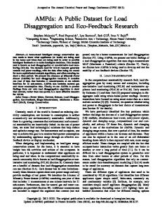
where Θ is the angle between voltage (V) and current (I). The power factor is unity (1) when the voltage and current are in phase and zero when the current leads or lags the voltage by 90 ◦ . Power factors are usually stated as leading or lagging to show the sign of the phase angle of current with respect to voltage. Table IV shows the result of an analysis we performed on 473,232 data point (per min readings) over 11 months. We found that real power readings had a high degree of fluctuation (as high as 10×, see Table IV) compared to current. This is due in part to the meter using two sensor readings (current and voltage) that can both fluctuate independently to measure real power. With BCPMs, current is measured on the same wire as the load while voltage is measured in one spot on the breaker power panel. There is a noticeable voltage drop when measuring voltage at the top of the breaker power panel vs the bottom. This means that if the BCPM meter is measuring the voltage level at a single spot the further away the current transformer (CT) the less accurate the voltage reading. This leads to a less accurate power reading when calculating the power associated to that CT. In addition, the resistiveness (R) of the load changes due to other factors such as wire gauge and material used. In other words, there is again a voltage drop from the breaker as compared to the plug outlet. It is worth noting that current is not affected by these problems. We concluded that using current would result in: (1) being better able to determine load states from historical data algorithmically, and (2) a higher classification accuracy score for the load disaggregation algorithm. Figure 4 shows the results from Table IV for the dishwasher. By examining the
B1E B2E BME CDE CWE DNE DWE EBE EQE FGE FRE GRE HPE HTE OFE OUE TVE UTE WOE
North Bedroom Master/South Br Basement Plugs & Lights Clothes Dryer Clothes Washer Dining Room Plugs Dishwasher Electronics Workbench Security/Network Kitchen Fridge HVAC/Furnace Garage Heat Pump Instant Hot Water Unit Home Office Outside Plug Ent TV/PVR/AMP Utility Room Plug Wall Oven
WHE UNE
Whole-House Meter Unmetered Loads
Distinct I
Distinct P
Flux
14 19 51 86 122 9 46 17 4 131 45 63 186 9 73 2 43 7 101
84 175 387 632 720 55 270 104 26 525 298 122 1268 70 408 6 415 24 646
6× 9× 8× 7× 6× 6× 6× 6× 7× 4× 7× 2× 7× 8× 6× 3× 10× 3× 6×
not tested not tested
750
500
250
0
0
100
200
300
Time (Minutes)
(a) 5 Hours of Real Power Consumption 3000
S3
S0
2500 S1 2000
Reads
Load
1500 S2
1000
500 0
0
0.5
1
1.5
2
2.5
3
3.5
4
4.5
5
5.5
6
6.5
7
750
800
854
Current (Amps)
(b) Distinct Current Measurements 3000 2500 2000
Reads
ID
Power (Watts)
1000
TABLE IV C URRENT vs R EAL P OWER C OMPARISON
1500 1000
500 0
0
50
100
150
200
250
300
350
400
450
500
550
600
650
700
Power (Watts)
(c) Distinct Real Power Measurements
number of distinct current reads (Figure 4(b)) we were able to algorithmically determine that the dishwasher had 4 finitestates. Figure 4(b) will form the basis for probability mass functions (PMF) that our load disaggregation algorithm will use. V. S INGLE -M EASUREMENT D ISAGGREGATION Using what we have discussed in the previous section, we continued to reflect on the nature of electrical systems and power. We know the following properties to hold true: (1) measurements of current draw are discrete as a limitation of the measuring device, (2) size of the breaker and/or the electrical limits of the load provide an upper bound on the measurements of current draw, and (3) zero is a lower bound on the measurements of current draw–current will never be negative. Load disaggregation research generally uses continuous probability distribution functions (e.g. Gaussian) [5], [6], [8] and generally ignores the idea of discrete probability. Zeifman [8] looks at a simple case of on/off appliances and appliance state transitions, but does not systematically analyze the single-measurement case. One potentially useful addition is to look at what can be inferred from a single measurement at a given time without analyzing the transitional probabilities (i.e. just by knowing the total current at that one time). Our single-measurement disaggregation algorithm uses discrete probabilities and single measurement to disaggregate all four types of appliances: simple on/off, finite-state, constantly on, and continuously variable [2]).
Fig. 4. An examination of the dishwasher. Comparing current (b) vs power (c) there is 6× as many different measurements for power as there is for current. This is due to fluctuations in voltage. Each spike in (b) can be seen as a distinct load/appliance state (4 states in the case of our dishwasher).
A. Formal Mathematical Model Let there be l independent discrete random variables X1 , X2 , . . . , Xl , corresponding to current draws from l loads. Each Xi is the deci-Ampere (dA) measurement of a metered electric load with a probability mass function (PMF) of pXi (x), where i is the load index i ∈ {1, 2, ..., l}, x is a number from a discrete set of possible measurements x ∈ {0, 1, ..., mi }, and mi is the upper bound imposed by the breaker that the i-th load is connected to. For example, with dA measurements on a 15A breaker, we would have mi = 150. The PMF pXi (x) is defined as follows: ( Pr[Xi = x], x ∈ {0, 1, . . . , mi }, pXi (x) = (2) 0, otherwise, where Pr[Xi = x] is the probability that the current draw of the i-th load is x. For example, if the PMF of Xi is (0.10, 0.05, 0.25, 0.40, 0.20, 0, 0, ...) for x ∈ {0, 1, 2, 3, 4, 5, 6, ...}, then Pr[Xi = 2] = 0.25, so the probability of the i-th load drawing 2 dA (i.e., 0.2 A) is 0.25. The probability Pr[Xi = x] is estimated from measurements over a sample period. For example, if over T measurements, the current draw x was recorded j times, then Pr[Xi = x] = j T . During the sample period each load is metered at a consistent rate of one measurement per minute. This rate determines the time resolution at which the load disaggregation will be
performed. Peaks in PMF pXi (x) are designated as probable load states s ∈ {0, 1, . . . , Si }, where Si + 1 is the number of states. The states are assigned by quantizing the range of possible measurements [0, mi ] (without gaps) so that each quantization bin contains one peak of the PMF. For example, in Figure 4(b), there are four peaks in the PMF, so we would model this PMF by a four-state model, with states being indexed {0, 1, 2, 3}. The probability of each state is the total probability mass within its quantization bin. B. MAP disaggregation A single measurement of the whole-house current draw is given by Z = X1 + X2 + ... + Xl , (3) where Z is the sum of current draws by all loads. We want to be able to determine the values of Xi ’s from the value of Z. In general, there are multiple combinations of Xi ’s that would produce any given Z, but not all of them have the same probability. We want to find the combination (X1 , X2 , ..., Xl ) that is the most probable, given the sum Z, i.e., the one that maximizes the posterior probability Pr(X1 , X2 , ..., Xl |Z). Note Plthat the conditional probability Pr(Z|X1 , X2 , ..., Xl ) = 1 if i=1 Xi = Z, and 0 otherwise, so by Bayes’ rule we have Pr(X1 , X2 , ..., Xl |Z) Pr(Z|X1 , X2 , ..., Xl )Pr(X1 , X2 , ..., Xl ) = Pr(Z) ( Pl Pr(X1 ,X2 ,...,Xl ) if i=1 Xi = Z, Pr(Z) = 0 else.
(4)
Since Pr(Z) is common to all combinations, it does not make a difference to their rank ordering in terms of probability. Hence, the MAP solution is the one P with the highest probl ability Pr(X1 , X2 , ..., Xl ) such that i=1 Xi = Z. Since the load current draws are assumed independent, we have Ql Pr(X1 , X2 , ..., Xl ) = i=1 Pr(Xi ). C. Experimental Setup and Results We chose 10 loads (or sub-meters) to disaggregate. Seven sub-meters containing a single load (CDE, CWE, DWE, FGE, FRE, HPE, WOE), 2 sub-meters containing multiple loads (BME, TVE) and the unmetered loads soft-meter (UNE). All loads can be considered finite-state loads. FRE (HVAC/Furnace) is mainly a constantly on load consisting of a fan and thermostat. CWE (Clothes Washer) is a front load washer with a variable speed spinning drum so it is a finitestate load combined with a continuously variable load. We ran the algorithm on the 524,544 current data points (per sub-meter) in AMPds. Ten experiments (one for each sub-meter) were run to see if single loads could be identified (or disaggregated) from the whole house reading. Accuracy is based on the correctness of both of: (1) the load being correctly identified, and (2) Ampere amount is the same as in the ground truth. We conducted our experiments using a Python implementation of the algorithm on a MacBook Air with a
1.8 GHz Core i7 CPU and 4 GB of memory. Table V shows our elapsed time and accuracy results which look promising. It currently takes ∼20 seconds to disaggregate all 10 loads for each time period. TABLE V L OAD D ISAGGREGATION R ESULTS ID
Load
BME CDE CWE DWE FGE FRE HPE TVE UNE WOE
Basement Plugs & Lights Clothes Dryer Clothes Washer Dishwasher Kitchen Fridge HVAC/Furnace Heat Pump Ent TV/PVR/AMP Unmetered Loads Wall Oven
Elapsed Time 23 16 33 19 32 21 30 20 48 18
minutes minutes minutes minutes minutes minutes minutes minutes minutes minutes
Accuracy 77.0% 97.9% 97.4% 97.3% 55.0% 33.8% 84.7% 57.0% 11.3% 99.5%
VI. T OWARDS R ICHER E CO -F EEDBACK Encouraging residents to consume less energy is key to conservation efforts; research indicates that simply improving the efficiency of how using one’s home can save between 10%–30% of energy [19]. However, the average person has a very difficult time understanding their energy use [19]–[21]. Both utilities (providers) and residents (consumers) are thus interested in residential eco-feedback [19] that offers residents both real-time and historical representations of their energy consumption. Currently available solutions tend to web-based simple analytical reports (http://myBCHydro.com portal) or R Insimple aggregate in-home displays (Rainforest ERT Home Display, TEDTM ). The success of these has been limited, with low utility and poor usability cited as common factors in low adoption [22]. An emerging field of visualization research focuses on what kinds of residential energy feedback are effective and appropriate, in which contexts, and in which locations [19]– [24]. Some of the critical research questions to examine in such eco-visualizations include temporal resolution (month, day, hour, minute) and presentation (real-time, historical); data scale (aggregate or detailed, multi-point or single-point); location (web-based, embedded in the home, mobile) and communicative intent (inform a tactical decision, support inferential analysis). The range of potential solutions spans a gamut from analytical, historical visualizations to real-time monitoring and at-a glance tactical feedback [20]–[22] but researchers are hampered by a paucity of readily accessible data at different resolutions and temporal scales. Commonly available data is typically either an aggregate total from a smart meter or a dataset of such values and timestamps provided in batch form and downloaded from the different utilities that supply electricity, natural gas, and water. This lack has motivated the development and publication of the dataset described in this paper.
Visualization and interaction researchers currently use this dataset for the design, development and testing of several prototype visualizations [23], [25], [26]. A variable feed at different temporal scales is embedded in a personal calendar showing the total energy use at different times [23], [27]. This uses near-real-time data (up to the last 10 minutes). A related approach represents the detailed house use by appliance and room, showing both the current use (kW) and the accumulated (kWh) for the day, in both traditional graphing and innovative informative art representations [25]. These feedback displays are intended for installation in a number of field sites beginning in 2014 in a longitudinal study in partnership with the provincial electricity utility. VII. C ONCLUSIONS We have presented AMPds a dataset that contains detailed measurements not seen in other datasets. In addition to power meter data we have also released water and natural gas meter data not done with other currently available datasets. We have also demonstrated the promising results of our initial load disaggregation algorithm. Unlike other load disaggregation algorithms ours can disaggregate all four types of appliances. Our future work includes augmenting our singlemeasurement disaggregation algorithm with a dynamics analysis (based on transitions) to improve the results. We are also looking at integrating the water and natural gas meter data as part of the disaggregation process to help identify multi-fuel appliances. We also see that the PMF created for each load can be used as a low frequency load signature which may be used to disaggregate appliances of the same make and model in other houses–an intuition that still needs to be tested. ACKNOWLEDGMENTS This work was supported in part by grants from the National Sciences and Engineering Research Council (NSERC) of Canada, along with the Graphics, Animation, and New Media Network of Centres of Excellence (GRAND NCE) of Canada. D OWNLOADING AMP DS AMPds is a free and publicly available dataset for all researchers to use, but any publishable research that makes use of this dataset must cite this paper. AMPds can be downloaded from: http://ampds.org/. R EFERENCES [1] F. Sultanem, “Using appliance signatures for monitoring residential loads at meter panel level,” Power Delivery, IEEE Transactions on, vol. 6, no. 4, pp. 1380–1385, 1991. [2] G. Hart, “Nonintrusive appliance load monitoring,” Proceedings of the IEEE, vol. 80, no. 12, pp. 1870–1891, 1992. [3] H. Kim, M. Marwah, M. Arlitt, G. Lyon, and J. Han, “Unsupervised disaggregation of low frequency power measurements,” in 11th International Conference on Data Mining, 2010, pp. 747–758. [4] J. Kolter, S. Batra, and A. Ng, “Energy disaggregation via discriminative sparse coding,” in Proc. Neural Information Processing Systems, 2010. [5] J. Kolter and T. Jaakkola, “Approximate inference in additive factorial hmms with application to energy disaggregation,” Journal of Machine Learning Research - Proceedings Track, vol. 22, pp. 1472–1482, 2012.
[6] O. Parson, S. Ghosh, M. Weal, and A. Rogers, “Non-intrusive load monitoring using prior models of general appliance types,” in TwentySixth Conference on Artificial Intelligence (AAAI-12), 2012. [7] M. Zeifman and K. Roth, “Nonintrusive appliance load monitoring: Review and outlook,” Consumer Electronics, IEEE Transactions on, vol. 57, no. 1, pp. 76–84, 2011. [8] M. Zeifman, “Disaggregation of home energy display data using probabilistic approach,” Consumer Electronics, IEEE Transactions on, vol. 58, no. 1, pp. 23 –31, 2012. [9] D. Bergman, D. Jin, J. Juen, N. Tanaka, C. Gunter, and A. Wright, “Nonintrusive load-shed verification,” IEEE Pervasive Computing, vol. 10, no. 1, pp. 49–57, 2011. [10] S. Makonin, F. Popowich, and B. Gill, “The Cognitive Power Meter: Looking Beyond the Smart Meter,” in Electrical and Computer Engineering (CCECE), 2013 26th IEEE Canadian Conference on, 2013, pp. 1–5. [11] S. Makonin and F. Popowich, “Home Occupancy Agent: Occupancy and Sleep Detection,” GSTF Journal on Computing, vol. 2, no. 1, pp. 182–186, 2012. [12] J. E. Fischer, S. D. Ramchurn, M. A. Osborne, O. Parson, T. D. Huynh, M. Alam, N. Pantidi, S. Moran, K. Bachour, S. Reece et al., “Recommending energy tariffs and load shifting based on smart household usage profiling,” in International Conference on Intelligent User Interfaces, 2013. [13] C. Beckel, L. Sadamori, and S. Santini, “Towards automatic classification of private households using electricity consumption data,” in Proceedings of the Fourth ACM Workshop on Embedded Sensing Systems for Energy-Efficiency in Buildings. ACM, 2012, pp. 169–176. [14] G.-y. Lin, S.-c. Lee, J.-J. Hsu, and W.-r. Jih, “Applying power meters for appliance recognition on the electric panel,” in Industrial Electronics and Applications (ICIEA), 2010 the 5th IEEE Conference on. IEEE, 2010, pp. 2254–2259. [15] J. Kolter and M. Johnson, “REDD: A Public Data Set for Energy Disaggregation Research,” in Workshop on Data Mining Applications in Sustainability (SIGKDD), San Diego, CA, 2011. [16] K. Anderson, A. Ocneanu, D. Benitez, D. Carlson, A. Rowe, and M. Berges, “BLUED: a fully labeled public dataset for Event-Based Non-Intrusive load monitoring research,” in 2012 Workshop on Data Mining Applications in Sustainability (SustKDD 2012), 2012. [17] S. Barker, A. Mishra, D. Irwin, E. Cecchet, P. Shenoy, and J. Albrecht, “Smart*: An open data set and tools for enabling research in sustainable homes,” in 2012 Workshop on Data Mining Applications in Sustainability (SustKDD 2012), 2012. [18] A. Reinhardt, P. Baumann, D. Burgstahler, M. Hollick, H. Chonov, M. Werner, and R. Steinmetz, “On the accuracy of appliance identification based on distributed load metering data,” in Sustainable Internet and ICT for Sustainability (SustainIT), 2012. IEEE, 2012, pp. 1–9. [19] S. Darby, “The effectiveness of feedback on energy consumption,” A Review for DEFRA of the Literature on Metering, Billing and direct Displays, vol. 486, 2006. [20] J. Rodgers and L. Bartram, “Exploring ambient and artistic visualization for residential energy use feedback,” Visualization and Computer Graphics, IEEE Transactions on, vol. 17, no. 12, pp. 2489–2497, 2011. [21] J. Froehlich, L. Findlater, and J. Landay, “The design of eco-feedback technology,” in Proceedings of the 28th international conference on Human factors in computing systems. ACM, 2010, pp. 1999–2008. [22] L. Bartram, J. Rodgers, and K. Muise, “Chasing the negawatt: visualization for sustainable living,” Computer Graphics and Applications, IEEE, vol. 30, no. 3, pp. 8–14, 2010. [23] D. Huang, L. Bartram, and M. Tory, “ConsumptionCalendar: Visualizing Resource Use in Context,” in Graphics, Animation and New Media Conference (GRAND), 2013. [24] G. Wood and M. Newborough, “Energy-use information transfer for intelligent homes: Enabling energy conservation with central and local displays,” Energy and Buildings, vol. 39, no. 4, pp. 495–503, 2007. [25] M. Sun and L. Bartram, “Informative Art for Energy Use Feedback,” in Graphics, Animation and New Media Conference (GRAND), 2013. [26] S. Makonin, M. Kashani, and L. Bartram, “The Affect of Lifestyle Factors on Eco-Visualization Design,” in Computer Graphics International (CGI), 2012, pp. 1–10. [27] R. S. Dembo and L. Bartram, “System and method for generating, processing and displaying data relating to consumption data with an application,” Mar. 21 2013, uS Patent 20,130,069,951.