A Two-Step Load Disaggregation Algorithm for Quasi-static Time-series Analysis on Actual Distribution Feeders Jiyu Wang, Xiangqi Zhu, David Mulcahy, Catie McEntee, David Lubkeman, and Ning Lu Electrical & Computer Engineering Department FREEDM Systems Center North Carolina State University, Raleigh, NC
[email protected]
Nader Samaan Pacific Northwest National Laboratory Richland, WA
Abstract—This paper focuses on developing a two-step load disaggregation method for conducting quasi-static time-series analysis using actual distribution feeder data. This can help utilities conduct power flow studies using smart meter measurements to assess the impact of high penetration of distributed energy resources. In the first step, load profiles of residential and commercial buildings obtained from smart meter data are used to match the load profile at the feeder head. This step will determine the number of residential and commercial loads on the feeder. The second step is to allocate the selected load profiles to each load node based on its transformer rating. This allows each load node to have its own load profile and the aggregation of those nodal load profiles matches closely to the metered feeder load shape at the substation. This algorithm is validated using smart meter data and the SCADA data of a real feeder. We compared the performance of the proposed method with the traditional load allocation method (i.e. use the feeder load shape for all subsequent load nodes scaling by the transformer capacities) when conducting quasi-static power flow studies. Results show that the proposed algorithm matches the utility data well and the obtained voltage profiles reveal more voltage dynamics than using the conventional load allocation method. Index Terms—Load disaggregation, load shape, quasi-static time-series analysis, distribution feeder, voltage profile
I. INTRODUCTION In recent years, the penetration of distributed energy resources (DER), such as controllable loads, roof-top PV and energy storage systems, are increasing rapidly [1-4]. Electric utilities need to evaluate the impact of DER integration on grid operation and planning [5-8]. Quasi-static time-series simulation [9] is now widely used to assess the operational characteristics (e.g. voltage profiles, overloading conditions, etc.) of an electricity distribution system [10-12]. A critical step in the Quasi-static time-series simulation is the allocation of nodal load profiles. In the past, the shape of the feeder head load profile is used for each subsequent load nodes and the load shape is scaled by letting its peak load be scaled based on the distribution transformer capacity at the node [13]. We refer to this method as the one-load-shape-scaling (OLSS) method.
Brant Werts and Andrew Kling Duke Energy Carolinas Charlotte, NC
The main disadvantage of this approach is all loads increase and decrease at the same time instance, making the modeling of voltage changes unrealistic. This approach is especially unfit when used for modeling the impact of PV penetration and demand response programs because the diversity of loads cannot be modeled and the PV penetration scenarios cannot be properly set up based on realistic estimation of the nodal loads. To improve the OLSS method, researchers proposed to use a few classes of load shapes. For example, by selecting two typical shapes for the residential load and one typical shape for the commercial load, one can make the allocation base on the customer types at each load node [14-15]. We refer to this approach as the multiple-load-shape-scaling method (MLSS). The MLSS method does not resolve the fundamental issue of the OLSS method as the load diversity cannot simply be modeled using a few typical load profiles. Electricity consumptions of residential and commercial buildings at distribution feeder level are highly random and can differ from each other drastically. The result of lacking load diversity is, when conducting quasistatic power flow studies, the actual voltage variations and ramping events are either under- or over- estimated. In [16-17], we proposed a load disaggregation method using a load profile database containing hundreds of load profiles. In this paper, we further developed the methodology. The paper has two major contributions. First, because we obtained a yearly utility feeder head load profile with the corresponding yearly smart meter data of all the residential and commercial buildings in the area, we are able to validate the performance of the algorithm by comparing the calculated number of houses and load types with the actual utility information. Second, we reformulated our load disaggregation algorithm into a 2-step algorithm that reflects the two main processes: load profile selection and allocation. The rest of the paper is organized as follows. Section II describes the load and feeder data used in this study. Section III introduces the detail of this load disaggregation algorithm. Case studies and the performance comparison with the OLSS method are discussed in Section IV. Conclusions and future works are included in Section V.
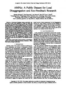
II. DATA PREPARATION An actual 12.47 kV distribution feeder is used in this study. The feeder has 995 nodes in total, within which, there are 454 load nodes. There are four voltage regulators and one 3-phase shunt capacitor with a capacity of 400 kvar. A set of metered feeder head load profiles are given with one-hour resolution collected from Jan 1st, 2016 to Dec 31st, 2016. Smart meter data collected from 5000 houses locate in the same state as the distribution feeder located are used to build the load profile database. The data resolution is 30-minute and the data were collected from Sep, 2015 to May, 2017. The loads include both residential and commercial. Profiles of a typical residential load in the area are plotted in Fig. 1. The first load peak occurs at around the wake-up and breakfast time around 7 a.m. and the second peak is the evening peak after the residents return home. Weekday and weekend loads are usually different as the residents’ schedule changes drastically over weekends. 12
Weekday Weekend
10
Load [kW]
8 6 4 2 0 5
0
10
15
20
Time [hour]
A. Load Profile Selection In the first step, we will select the combination of the residential and commercial load profiles that can provide a best match to the feeder head load profiles. A multi-pivot-points matching (MPPM) method is used to find the load profiles from the load profile database so that the aggregated load profile matches the feeder head load profile. Because the peak load is usually the most important point in the 48 points on the feeder head load profile, the single-pivotpoint matching (SPPM) method uses the peak load point, 𝑝𝑝𝑝𝑝𝑝𝑝𝑝𝑝 𝑝𝑝𝑝𝑝𝑝𝑝𝑝𝑝 (𝑃𝑃𝑓𝑓𝑓𝑓𝑓𝑓𝑓𝑓𝑓𝑓𝑓𝑓 , 𝑡𝑡𝑓𝑓𝑓𝑓𝑓𝑓𝑓𝑓𝑓𝑓𝑓𝑓 ), as the pivot. The matching criterion are 𝑎𝑎𝑎𝑎𝑎𝑎
(1 + 𝑘𝑘) ≥
20
Weekday
(1 + 𝑘𝑘) ≥
Load [kW]
𝑎𝑎𝑎𝑎𝑎𝑎
𝑝𝑝𝑝𝑝𝑝𝑝𝑝𝑝
𝑃𝑃𝑓𝑓𝑓𝑓𝑓𝑓𝑓𝑓𝑓𝑓𝑓𝑓�𝑡𝑡=𝑡𝑡𝑓𝑓𝑓𝑓𝑓𝑓𝑓𝑓𝑓𝑓𝑓𝑓� 𝑎𝑎𝑎𝑎𝑎𝑎𝑎𝑎𝑎𝑎𝑎𝑎𝑎𝑎
𝑃𝑃𝑓𝑓𝑓𝑓𝑓𝑓𝑓𝑓𝑓𝑓𝑓𝑓
𝑎𝑎𝑎𝑎𝑎𝑎𝑎𝑎𝑎𝑎𝑎𝑎𝑎𝑎
≥ (1 − 𝑘𝑘)
(3) (4)
𝑝𝑝𝑝𝑝𝑝𝑝𝑝𝑝
𝑡𝑡𝑓𝑓𝑓𝑓𝑓𝑓𝑓𝑓𝑓𝑓𝑓𝑓 : Load peaking time of the actual feeder head load
Note that criterion (3) and (4) are used to guarantee the the 𝑝𝑝𝑝𝑝𝑝𝑝𝑝𝑝 simulated feeder head profile is peaked at 𝑡𝑡𝑓𝑓𝑓𝑓𝑓𝑓𝑓𝑓𝑓𝑓𝑓𝑓 . For a nonpeak pivot point, the matching criterion are simply 𝑎𝑎𝑎𝑎𝑎𝑎 𝑗𝑗 𝑃𝑃𝑓𝑓𝑓𝑓𝑓𝑓𝑓𝑓𝑓𝑓𝑓𝑓 �𝑡𝑡𝑓𝑓𝑓𝑓𝑓𝑓𝑓𝑓𝑓𝑓𝑓𝑓 � 𝑎𝑎𝑎𝑎𝑎𝑎
𝑗𝑗
= � 𝑃𝑃𝑖𝑖 �𝑡𝑡 = 𝑡𝑡𝑓𝑓𝑓𝑓𝑓𝑓𝑓𝑓𝑓𝑓𝑓𝑓 �
𝑃𝑃𝑓𝑓𝑓𝑓𝑓𝑓𝑓𝑓𝑓𝑓𝑓𝑓 𝑗𝑗
𝑁𝑁
𝑃𝑃𝑓𝑓𝑓𝑓𝑓𝑓𝑓𝑓𝑓𝑓𝑓𝑓
𝑖𝑖=1
≥ (1 − 𝑘𝑘)
A match is not reached if
10
(2)
𝑝𝑝𝑝𝑝𝑝𝑝𝑝𝑝
Chritmas Black Friday
≥ (1 − 𝑘𝑘)
(1)
𝑃𝑃𝑓𝑓𝑓𝑓𝑓𝑓𝑓𝑓𝑓𝑓𝑓𝑓 : Peak of the actual feeder head load
Thanksgiving
15
𝑝𝑝𝑝𝑝𝑝𝑝𝑝𝑝
𝑖𝑖𝑖𝑖{1, … , 𝑁𝑁} where 𝑁𝑁: Number of loads in this feeder 𝑃𝑃𝑖𝑖 : Load profile of house 𝑖𝑖 on the selected day 𝑘𝑘: Error bound (a typical value of 𝑘𝑘 is 0.001) 𝑎𝑎𝑎𝑎𝑎𝑎𝑎𝑎𝑎𝑎𝑎𝑎𝑎𝑎 𝑃𝑃𝑓𝑓𝑓𝑓𝑓𝑓𝑓𝑓𝑓𝑓𝑓𝑓 : Peak of the simulated feeder head load profile 𝑎𝑎𝑎𝑎𝑎𝑎 𝑃𝑃𝑓𝑓𝑓𝑓𝑓𝑓𝑓𝑓𝑓𝑓𝑓𝑓 : Aggregated load profile
(1 + 𝑘𝑘) ≥
Weekend
𝑎𝑎𝑎𝑎𝑎𝑎 𝑃𝑃𝑓𝑓𝑓𝑓𝑓𝑓𝑓𝑓𝑓𝑓𝑓𝑓 𝑝𝑝𝑝𝑝𝑝𝑝𝑝𝑝 𝑃𝑃𝑓𝑓𝑓𝑓𝑓𝑓𝑓𝑓𝑓𝑓𝑓𝑓
𝑁𝑁 max(∑𝑁𝑁 𝑖𝑖=1 𝑃𝑃𝑖𝑖 (𝑡𝑡 = 1) , … , ∑𝑖𝑖=1 𝑃𝑃𝑖𝑖 (𝑡𝑡 = 48)) = 𝑃𝑃𝑓𝑓𝑓𝑓𝑓𝑓𝑓𝑓𝑓𝑓𝑓𝑓
Fig. 1. Monthly energy consumption for a residential house
Profiles of a commercial load are plotted in Fig. 2. Commercial loads usually have a higher consumption between 9 a.m. to 8 p.m. During holidays such as Thanksgiving and Christmas, most commercial loads will shift significantly from its regular consumption patterns.
𝑝𝑝𝑒𝑒𝑎𝑎𝑎𝑎
𝑃𝑃𝑓𝑓𝑓𝑓𝑓𝑓𝑓𝑓𝑓𝑓𝑓𝑓 �𝑡𝑡 = 𝑡𝑡𝑓𝑓𝑓𝑓𝑓𝑓𝑓𝑓𝑓𝑓𝑓𝑓 � = ∑𝑁𝑁 𝑖𝑖=1 𝑃𝑃𝑖𝑖 �𝑡𝑡 = 𝑡𝑡𝑓𝑓𝑓𝑓𝑓𝑓𝑓𝑓𝑓𝑓𝑓𝑓 �
𝑎𝑎𝑎𝑎𝑎𝑎
𝑃𝑃𝑓𝑓𝑓𝑓𝑓𝑓𝑓𝑓𝑓𝑓𝑓𝑓 𝑗𝑗
𝑃𝑃𝑓𝑓𝑓𝑓𝑓𝑓𝑓𝑓𝑓𝑓𝑓𝑓
> (1 + 𝑘𝑘).
(5)
(6)
The aggregation algorithm for the MPPM method is: 5
Algorithm 1 MPPM Algorithm 1:
0 0
5
10
15
20
Time [hour]
Fig. 2. Monthly energy consumption for a commercial house
The two examples show that if realistic load profiles of residential and commercial buildings are used in the simulation, the impacts of load pattern shifts can be modeled more realistically.
2:
3:
4:
III. LOAD DISAGGREGATION ALGORITHM This section introduces the detail of the load disaggregation algorithm. The algorithm has two steps: load profile selection and load allocation to each load nodes. 5:
Construct a load profile database using 5000 smart meter data collected in the same geographical area as the distribution feeder located. Select the pivot feeder head load profile to match. For example, we selected the metered feeder head load profile in the 𝑗𝑗𝑡𝑡ℎ day to be the target load profile to match. Select 𝑚𝑚 pivot points on the pivot load profile for matching and one of the pivot point is the peak load of the day. So we have 𝑚𝑚 pairs of non𝑗𝑗 𝑗𝑗 peak pivot points �𝑃𝑃𝑓𝑓𝑓𝑓𝑓𝑓𝑓𝑓𝑓𝑓𝑓𝑓 , 𝑡𝑡𝑓𝑓𝑓𝑓𝑓𝑓𝑓𝑓𝑓𝑓𝑓𝑓 � with 𝑗𝑗𝑗𝑗{1, … , 𝑚𝑚} and one peak load 𝑝𝑝𝑝𝑝𝑝𝑝𝑝𝑝
𝑝𝑝𝑝𝑝𝑝𝑝𝑝𝑝
point (𝑃𝑃𝑓𝑓𝑓𝑓𝑓𝑓𝑓𝑓𝑓𝑓𝑓𝑓 , 𝑡𝑡𝑓𝑓𝑓𝑓𝑓𝑓𝑓𝑓𝑓𝑓𝑓𝑓 ). Match the peak load point using (1)-(4). for 𝑖𝑖 = 1: 5000 𝑗𝑗 𝑖𝑖 Randomly select �𝑃𝑃𝑙𝑙𝑙𝑙𝑙𝑙𝑙𝑙 , 𝑡𝑡𝑓𝑓𝑓𝑓𝑓𝑓𝑓𝑓𝑓𝑓𝑓𝑓 � from the load database. Use (1)-(4) to check the match. If a match is reached, keep all the load profiles and end the iteration. If a match is not reached, repeat the process. end Check to see if the other non-peak load pivot points matches using (5)(6). If “yes”, end the process. If “no”, repeat Step 4.
By aggregating the load profiles until the error between the peak of the aggregated load profile and metered data reaches the acceptable limit, we can obtain the number of houses in this feeder as well as a diversified group of load. A few rules reflecting the feeder characteristics are set to guarantee that a good match can be achieved. This requires a statistic analysis of the typical distribution feeder in the area. For example, a maximum number of large load rule is in placed to 𝐿𝐿𝐿𝐿𝐿𝐿𝐿𝐿𝐿𝐿𝐿𝐿 ≤ limit the number of large load (defined by 𝑃𝑃𝑙𝑙𝑙𝑙𝑙𝑙𝑙𝑙𝑙𝑙𝑙𝑙𝑙𝑙𝑙𝑙𝑙𝑙
week is plotted in Fig. 5. The matching day is Day 5 with 3 pivot points and it can be observed that the two profiles in that day has the best match. In other days although sometimes there will be a difference but the overall weekly shape is the same. Table I summarizes the comparison results with the actual feeder head loads in seven days. 250
200
𝐴𝐴𝐴𝐴 =
24 ∑7 𝑑𝑑𝑑𝑑𝑑𝑑=1(∑𝑡𝑡=1
𝐴𝐴𝐴𝐴𝐴𝐴 =
𝑎𝑎𝑎𝑎𝑎𝑎 �𝑃𝑃𝑎𝑎𝑎𝑎𝑎𝑎𝑎𝑎𝑎𝑎𝑎𝑎 𝑓𝑓𝑓𝑓𝑓𝑓𝑓𝑓𝑓𝑓𝑓𝑓 (𝑑𝑑𝑑𝑑𝑑𝑑,𝑡𝑡)−𝑃𝑃𝑓𝑓𝑓𝑓𝑓𝑓𝑓𝑓𝑓𝑓𝑓𝑓 (𝑑𝑑𝑑𝑑𝑑𝑑,𝑡𝑡)� ) (𝑡𝑡) 𝑃𝑃𝑎𝑎𝑎𝑎𝑎𝑎𝑎𝑎𝑎𝑎𝑎𝑎 𝑓𝑓𝑓𝑓𝑓𝑓𝑓𝑓𝑓𝑓𝑓𝑓
7×24
𝑎𝑎𝑎𝑎𝑎𝑎 �𝑃𝑃𝑎𝑎𝑎𝑎𝑎𝑎𝑎𝑎𝑎𝑎𝑎𝑎 𝑓𝑓𝑓𝑓𝑓𝑓𝑓𝑓𝑓𝑓𝑓𝑓 (𝑑𝑑𝑑𝑑𝑑𝑑,𝑡𝑡)−𝑃𝑃𝑓𝑓𝑓𝑓𝑓𝑓𝑓𝑓𝑓𝑓𝑓𝑓 (𝑑𝑑𝑑𝑑𝑑𝑑,𝑡𝑡))� ) (𝑡𝑡) 𝑃𝑃𝑎𝑎𝑎𝑎𝑎𝑎𝑎𝑎𝑎𝑎𝑎𝑎 𝑓𝑓𝑓𝑓𝑓𝑓𝑑𝑑𝑑𝑑𝑑𝑑
24 ∑7 𝑑𝑑𝑑𝑑𝑑𝑑=1(∑𝑡𝑡=1
7×24
100
50
470
500
550
525
580
610
635
Number of house selected
Fig. 3. Histogram for number of houses for 100 simulations in one day 650
Number of houses selected
B. Consistency of the Results of Load Profile Selection After each valid matching, a group of load profiles is obtained, so we need to estimate which group of profiles can provide a best overall match. We ran the algorithm 100 times for matching a daily feeder head load profile. The number of houses selected at each run is summarized in Fig. 3. The mean number is 551, the maximum number 649 and the minimum number is 455. Although the number of houses varies in each iteration, extreme conditions where too many small or large houses are selected can be excluded. Fig. 4 shows the boxplot of the simulation results when we select 7 daily profiles and for each profile, we run the algorithm for 100 to receive 100 successful matching load groups. For most of the days, the mean number of loads selected is 551. The actual number of loads on the feeder is 590. The difference is approximately 6%. This difference can be further reduced if we limit the amount of big loads being selected. Note that because the load database consists of house in the general area but not exactly the load supplied by this particular distribution feeder, it is impossible to achieve 100% match. The next step is to decide which load groups provide a better match for all seven daily load profiles. The average error, 𝐴𝐴𝐴𝐴, and the average absolute error, 𝐴𝐴𝐴𝐴𝐴𝐴, are calculated as
150
0
600
550
500
450 Day 1
Day 2
Day 3
Day 4
Day 5
Day 6
Day 7
Fig. 4. Boxplot for number of houses in seven days Day 2
Day 1
1600
Day 4
Day 3
Day 5
Day 6
Matching
Day 7
Pivot point 1
Day
1400 1200
Load [kW]
𝑗𝑗
25 and 𝑁𝑁𝑙𝑙𝑙𝑙𝑙𝑙𝑙𝑙𝑙𝑙𝑙𝑙𝑙𝑙𝑙𝑙𝑙𝑙 = 1. For the other loads, we let 𝑃𝑃𝑙𝑙𝑙𝑙𝑙𝑙𝑙𝑙 ≤ 20. Thus, we only select one house that has a maximum power between 20-25 kW. This constraint is used to make sure that that the aggregated energy consumption for each load node is smaller than the distribution transformer rating.
Number of occurrence
𝐻𝐻𝐻𝐻𝐻𝐻ℎ𝑙𝑙𝑙𝑙𝑙𝑙
𝑖𝑖 𝑀𝑀𝑀𝑀𝑀𝑀 𝑃𝑃𝑙𝑙𝑙𝑙𝑙𝑙𝑙𝑙𝑙𝑙𝑙𝑙𝑙𝑙𝑙𝑙𝑙𝑙 ≤ 𝑃𝑃𝑙𝑙𝑙𝑙𝑙𝑙𝑙𝑙𝑙𝑙𝑙𝑙𝑙𝑙𝑙𝑙𝑙𝑙 ) being selected to 𝑁𝑁𝑙𝑙𝑙𝑙𝑙𝑙𝑙𝑙𝑙𝑙𝑙𝑙𝑙𝑙𝑙𝑙𝑙𝑙 . This rule selects large houses based on the number of large load nodes on the feeder to make sure only a limited amount of large loads are selected and can be placed to those nodes. On the feeder we selected for illustrate the method in this paper, there is only one load node with a distribution transformer 𝑗𝑗 capacity greater than 25 kVA. Thus, we set 20 ≤ 𝑃𝑃𝑙𝑙𝑙𝑙𝑙𝑙𝑙𝑙𝑙𝑙𝑙𝑙𝑙𝑙𝑙𝑙𝑙𝑙 ≤
Pivot point 3
1000 800 600 Pivot point 2
400 0
48
24 Metered Feeder Head Profile Aggregated Feeder Head Profile
72
120
96
144
168
Time [hour]
Fig. 5. Feeder head profile comparison Table I. Feeder head profile aggregation summary 0.88% 5.21% 1406.2 kW 0.094% 552
Average Error Average Absolute Error Peak Load Peak load Error Total Number of houses
(7)
(8)
All load groups resulting a total number of loads between 540 and 560 are selected. Their aggregated load profiles are compared with the other six daily profiles. The load group with the lowest 𝐴𝐴𝐴𝐴 and 𝐴𝐴𝐴𝐴𝐴𝐴 values are selected. This load group consists of 552 houses and the aggregated load profile in one
C. Load Allocation to Each Load Node At this step, we need to allocate the 552 load profiles to each load node based on the distribution transformer rating. Therefore, the power allocation for each load node, 𝑃𝑃𝑖𝑖𝑎𝑎𝑎𝑎𝑎𝑎𝑎𝑎𝑎𝑎𝑎𝑎𝑎𝑎𝑎𝑎𝑎𝑎 , is calculated as 𝑃𝑃𝑖𝑖𝑎𝑎𝑎𝑎𝑎𝑎𝑎𝑎𝑎𝑎𝑎𝑎𝑎𝑎𝑎𝑎𝑎𝑎 =
𝑝𝑝𝑝𝑝𝑝𝑝𝑘𝑘
𝑋𝑋𝑋𝑋𝑋𝑋𝑋𝑋𝑋𝑋𝑖𝑖 ∗𝑃𝑃𝑓𝑓𝑓𝑓𝑓𝑓𝑓𝑓𝑓𝑓𝑓𝑓 𝑁𝑁
𝑛𝑛𝑛𝑛𝑛𝑛𝑛𝑛 𝑋𝑋𝑋𝑋𝑋𝑋𝑋𝑋𝑋𝑋 ∑𝑗𝑗=1 𝑗𝑗
𝑖𝑖 ∈ {1,2, … , 𝑁𝑁𝑛𝑛𝑛𝑛𝑛𝑛𝑛𝑛 }
(9)
where 𝑋𝑋𝑋𝑋𝑋𝑋𝑋𝑋𝑋𝑋𝑖𝑖 is the distribution transformer KVA rating at node 𝑖𝑖 and 𝑁𝑁𝑛𝑛𝑛𝑛𝑛𝑛𝑛𝑛 is the number of load nodes on the feeder. After 𝑃𝑃𝑖𝑖𝑎𝑎𝑎𝑎𝑎𝑎𝑎𝑎𝑎𝑎𝑎𝑎𝑎𝑎𝑎𝑎𝑎𝑎 is calculated for all load nodes, we allocate the load profiles to each nodes to calculate the aggregated load at the load node by 𝑁𝑁𝑙𝑙𝑙𝑙𝑙𝑙𝑙𝑙,𝑖𝑖 𝑎𝑎𝑎𝑎𝑎𝑎𝑎𝑎𝑎𝑎𝑎𝑎𝑎𝑎𝑎𝑎𝑎𝑎𝑎𝑎 𝑝𝑝𝑝𝑝𝑝𝑝𝑝𝑝 = ∑𝑗𝑗=1 𝑃𝑃𝑗𝑗 �𝑡𝑡𝑓𝑓𝑓𝑓𝑓𝑓𝑓𝑓𝑓𝑓𝑓𝑓 � (10) 𝑃𝑃𝑖𝑖 𝑗𝑗 ∈ �1,2, … , 𝑁𝑁𝑙𝑙𝑙𝑙𝑙𝑙𝑙𝑙,𝑖𝑖 � The number of the loads at node 𝑖𝑖, 𝑁𝑁𝑙𝑙𝑙𝑙𝑙𝑙𝑙𝑙,𝑖𝑖 , is determined by (1 + 𝑘𝑘) ≥
𝑎𝑎𝑎𝑎𝑎𝑎𝑎𝑎𝑎𝑎𝑎𝑎𝑎𝑎𝑎𝑎𝑎𝑎𝑎𝑎 𝑃𝑃𝑖𝑖 𝑃𝑃𝑖𝑖𝑎𝑎𝑎𝑎𝑎𝑎𝑎𝑎𝑎𝑎𝑎𝑎𝑎𝑎𝑎𝑎𝑎𝑎
≥ (1 − 𝑘𝑘)
𝑎𝑎𝑎𝑎𝑎𝑎𝑎𝑎𝑎𝑎𝑎𝑎𝑎𝑎𝑎𝑎𝑎𝑎𝑎𝑎
�𝑃𝑃𝑖𝑖𝑎𝑎𝑎𝑎𝑎𝑎𝑎𝑎𝑎𝑎𝑎𝑎𝑎𝑎𝑎𝑎𝑎𝑎 −𝑃𝑃𝑖𝑖
𝑃𝑃𝑖𝑖𝑎𝑎𝑎𝑎𝑎𝑎𝑎𝑎𝑎𝑎𝑎𝑎𝑎𝑎𝑎𝑎𝑎𝑎
�
(12)
The nodal load allocation algorithm is summarized as follows: Algorithm 2 Nodal Load Allocation Algorithm 1: 2: 3:
4: 5:
454 0% 2.13% 3
Total Load Nodes Average Error Average Absolute Error Node with abs error>5% 10 Aggregated Load Profile at One Node
8
Three houses locate at this node Load Profile for each house
6
(11)
where 𝑘𝑘 is an error band with a typical value of 0.05. We allocate 552 load profiles to each node following an ascending order. This means we start from allocating the load profiles to the smallest load node first. Note that if a random order or a descending order is followed, large nodes may have been allocated with too many small loads at the beginning of the process. Then, in the end, there are insufficient small loads left to fit in the small load nodes. Towards the end of the matching, if there is no load left to be dispatched to the remaining nodes, we will change the lower limit (1 − 𝑘𝑘) of the matching criteria (11) to a smaller value. For example, 𝑘𝑘 can reduced from 0.95 to 0.9. Note that a typical value of 𝑘𝑘 is 0.05. This will result in fewer houses being allocated to each node. If there is a few loads left, we will place the leftover loads to the nodes so that the least percentage errors, 𝑃𝑃𝑃𝑃, after adding in one more load is the least. 𝑃𝑃𝑃𝑃 =
Table II. House disaggregation summary
Import the load group of 𝑁𝑁 loads from the result of the MPPM algorithm. Calculate 𝑃𝑃𝑖𝑖𝑎𝑎𝑎𝑎𝑎𝑎𝑎𝑎𝑎𝑎𝑎𝑎𝑎𝑎𝑎𝑎𝑎𝑎 for each node base on (9) and sort 𝑃𝑃𝑖𝑖𝑎𝑎𝑎𝑎𝑎𝑎𝑎𝑎𝑎𝑎𝑎𝑎𝑎𝑎𝑎𝑎𝑎𝑎 in ascending order. for 𝑖𝑖=1:𝑁𝑁𝑛𝑛𝑛𝑛𝑛𝑛𝑛𝑛 Starting with the node with the least 𝑃𝑃𝑖𝑖𝑎𝑎𝑎𝑎𝑎𝑎𝑎𝑎𝑎𝑎𝑎𝑎𝑎𝑎𝑎𝑎𝑎𝑎 if 𝑁𝑁 = 0 𝑘𝑘 = 𝑘𝑘 − 0.05 and repeat step 3 end While (true) Draw one load from the load pool with 𝑁𝑁 loads 𝑎𝑎𝑎𝑎𝑎𝑎𝑎𝑎𝑎𝑎𝑎𝑎𝑎𝑎𝑎𝑎𝑎𝑎𝑎𝑎 Calculate 𝑃𝑃𝑖𝑖 use (10) 𝑎𝑎𝑎𝑎𝑎𝑎𝑎𝑎𝑎𝑎𝑎𝑎𝑎𝑎𝑎𝑎𝑎𝑎𝑎𝑎 / 𝑃𝑃𝑖𝑖𝑎𝑎𝑎𝑎𝑎𝑎𝑎𝑎𝑎𝑎𝑎𝑎𝑎𝑎𝑎𝑎𝑎𝑎 < (1 − 𝑘𝑘) if 𝑃𝑃𝑖𝑖 𝑎𝑎𝑎𝑎𝑎𝑎𝑎𝑎𝑎𝑎𝑎𝑎𝑎𝑎𝑎𝑎𝑎𝑎𝑎𝑎 / 𝑃𝑃𝑖𝑖𝑎𝑎𝑎𝑎𝑎𝑎𝑎𝑎𝑎𝑎𝑎𝑎𝑎𝑎𝑎𝑎𝑎𝑎 > (1 + 𝑘𝑘) else if 𝑃𝑃𝑖𝑖 𝑎𝑎𝑎𝑎𝑎𝑎𝑎𝑎𝑎𝑎𝑎𝑎𝑎𝑎𝑎𝑎𝑎𝑎𝑎𝑎 =0 𝑃𝑃𝑖𝑖 else save the load profiles for Node 𝑖𝑖 update the load pool to 𝑁𝑁 = 𝑁𝑁 − 𝑁𝑁𝑙𝑙𝑙𝑙𝑙𝑙𝑙𝑙,𝑖𝑖 break the while loop end end end Place the leftover loads to the nodes with lowest PE until no load left. Record all the load profiles and house IDs for all nodes in this feeder.
The statistics of the house disaggregation result is summarized in Table II and an example of the aggregated load profile is shown in Fig. 6.
4
2
0 0
5
10
15
20
25
Fig. 6. An example of load allocation disaggregation at a load node
IV. SIMULATION RESULTS This section presents the simulation results. Voltage profiles from the MPPM method is compared with the OLSS method when running a monthly quasi-static time-series simulation using OpenDSS. To compare the impact of using different load shapes at each load node on feeder load profile, we disabled all voltage regulators during simulation. We run a 31-day simulation with half-hour data resolution. Therefore, 1488 power flow runs are conducted to obtain the voltage profiles at each node for the 31day period. To compare the differences between the simulation results obtained by the two methods, we compared the two load shapes by calculating the average voltage difference percentage for node 𝑖𝑖, 𝑃𝑃𝑃𝑃𝑃𝑃𝑖𝑖 , using 𝑃𝑃𝑃𝑃𝑃𝑃𝑖𝑖 =
𝑢𝑢 �(𝑉𝑉𝑑𝑑 𝑖𝑖 (𝑡𝑡)−𝑉𝑉𝑖𝑖 (𝑡𝑡)� (𝑡𝑡) 𝑉𝑉𝑑𝑑 𝑖𝑖
∑1488 𝑡𝑡=1
1488
× 100%
(13)
𝑖𝑖 ∈ {1,2, … , 𝑁𝑁} where 𝑉𝑉𝑖𝑖𝑀𝑀𝑀𝑀𝑀𝑀𝑀𝑀 (𝑡𝑡) and and 𝑉𝑉𝑖𝑖𝑂𝑂𝑂𝑂𝑂𝑂𝑂𝑂 (𝑡𝑡) are the voltage calculated at node 𝑖𝑖 using MPPM and OLSS method, respectively. The 𝑃𝑃𝑃𝑃𝑃𝑃 versus the distance from feeder head to each node is plotted in Fig. 7. The results show that the average voltage differences are getting larger and larger as the nodes are further away from the feeder head. The largest difference is 78 V on a between the results obtained by the two methods. The location is at the feeder end of phase B. Phase A has the smallest voltage difference at the feeder end and it is still 24 V. Note that the data resolution is 30-minute in this study, so the voltage difference is underrated because the average power variation are much larger for 15-minute data. This shows that the voltage difference is at least 3-5 times bigger if minute-byminute data is used. More details about the comparison of the two methods will be presented in our follow-up journal paper.
1.2
ACKNOWLEDGEMENT
Phase A Phase B
Average V difference PCT
1
Phase C
0.8 0.6 0.4 0.2 0 4
2
0
6
8
10
12
14
Distance to feeder head
This study is funded by the U.S. Department of Energy SunShot Initiative and Center for Advanced Power Engineering Research (CAPER). The project team wants to especially thank Dr. Guohui Yuan, Dr. Kemal Celik, Ms. Rebecca Hott, and Mr. Jeremiah Miller from the Systems Integration Subprogram at the Department of Energy SunShot Initiative for their continuing support, help, and guidance. The authors would also like to thank Steve Whisenant and John Gajda at Duke Energy for providing the team with the data and feedback. REFERENCES
Fig. 7. Voltage difference percentage for three phases
Fig. 8 is the boxplot showing the distribution of the voltage differences at different time-of-the-day for all nodes. In general, the voltage difference during daytime is larger as the power consumption is higher. From the preliminary results, we observed that it is important to model each node using realistic load shapes. If the same load shape is applied to each node, the modeling of voltage and power flow will differ from the actual cases, especially for the peak loading conditions and for nodes at feeder end.
[1] [2] [3]
[4]
[5]
1
Average V difference PCT
[6] 0.8
0.6
[7]
0.4
[8]
0.2 1
2
3
4
5
6
7
8
9
10 11 12 13 14 15 16 17 18 19 20 21 22 23 24
Hour
Fig. 8. Boxplot of voltage difference at different time
[9]
[10]
V. CONCLUSION AND FUTURE WORK This paper presents a two-step MPPM load disaggregation algorithm for conducting quasi-static time-series simulation on actual distribution feeder using realistic smart meter data and the substation feeder head load profiles. The smart meter data can be used to develop a load profile database. In the first step, to populate the load nodes with realistic load profiles, the MPPM disaggregation algorithm use multiple pivot points to provide a reasonable match for the aggregated load to the feeder head load profiles. Through this process, the number of loads are determined and a group of loads that can provide the best fit will be selected to proceed to the second step, the nodal load allocation step. Based on the distribution transformer capacities, a load allocation algorithm is proposed to produce reasonable nodal load profiles for each nodes. The simulation results demonstrate that compared with the ongoing approach, this method produces more realistic voltage and power flow results that match the measurements at the feeder well. A comprehensive comparison of the performance of the MPPM algorithm with other existing approach will be published in our follow-up journal articles.
[11]
[12]
[13]
[14]
[15]
[16]
[17]
Solangi, K. H., et al. "A review on global solar energy policy." Renewable and sustainable energy reviews 15.4 (2011): 2149-2163. Birol, Fatih. "World energy outlook." Paris: International Energy Agency 23.4 (2008): 329. Hand, M. M., et al. Renewable Electricity Futures Study. Volume 1. Exploration of High-Penetration Renewable Electricity Futures. No. NREL/TP--6A20-52409-1. National Renewable Energy Lab.(NREL), Golden, CO (United States), 2012. Cappers, Peter, Charles Goldman, and David Kathan. "Demand response in US electricity markets: Empirical evidence." Energy35.4 (2010): 1526-1535. Alam, M. J. E., K. M. Muttaqi, and D. Sutanto. "Effectiveness of traditional mitigation strategies for neutral current and voltage problems under high penetration of rooftop PV." Power and Energy Society General Meeting (PES), 2013 IEEE. IEEE, 2013. Solanki, Sarika Khushalani, Vaidyanath Ramachandran, and Jignesh Solanki. "Steady state analysis of high penetration PV on utility distribution feeder." Transmission and Distribution Conference and Exposition (T&D), 2012 IEEE PES. IEEE, 2012. Zhu, Xiangqi, Jiahong Yan, and Ning Lu. "A Graphical PerformanceBased Energy Storage Capacity Sizing Method for High Solar Penetration Residential Feeders." IEEE Transactions on Smart Grid 8.1 (2017): 3-12. Ke, Xinda, Ning Lu, and Chunlian Jin. "Control and size energy storage systems for managing energy imbalance of variable generation resources." IEEE Transactions on Sustainable Energy 6.1 (2015): 70-78. IEEE P1547.7 D5.1 Draft Guide to Conducting Distribution Impact Studies for Distributed Resource Interconnection, IEEE Standard, Aug. 2011. Ke, Xinda, et al. "A Three-Stage Enhanced Reactive Power and Voltage Optimization Method for High Penetration of Solar." the Proc. of IEEE/PES General Meeting. 2017. Zhu, Xiangqi, et al. "Voltage-Load Sensitivity Matrix Based Demand Response for Voltage Control in High Solar Penetration Distribution Feeders." Power & Energy Society General Meeting, 2017 IEEE. IEEE, 2017. Mozina, Charles J. "Impact of smart grid and green power generation on distribution systems." Innovative Smart Grid Technologies (ISGT), 2012 IEEE PES. IEEE, 2012. Jardini, J. A., et al. "Distribution transformer loading evaluation based on load profiles measurements." IEEE Transactions on Power Delivery 12.4 (1997): 1766-1770. Mather, Barry A. "Quasi-static time-series test feeder for PV integration analysis on distribution systems." Power and Energy Society General Meeting, 2012 IEEE. IEEE, 2012. Zhu, Xiangqi, Jiahong Yan, and Ning Lu. "A probabilistic-based PV and energy storage sizing tool for residential loads." Transmission and Distribution Conference and Exposition (T&D), 2016 IEEE/PES. IEEE, 2016. Wang, Jiyu, et al. "Continuation power flow analysis for PV integration studies at distribution feeders." Power & Energy Society Innovative Smart Grid Technologies Conference (ISGT), 2017 IEEE. IEEE, 2017. Wang, Jiyu, et al. “Load aggregation methods for quasi-static power flow analysis on high PV penetration feeders.” Transmission and Distribution Conference and Exposition (T&D), 2018 IEEE/PES, in press.