Amplifying the Block Matrix Structure for Spectral Clustering - CiteSeerX

Amplifying the Block Matrix Structure for Spectral Clustering

Igor Fischer Telecommunications Lab Saarland University 22.10 P.O. Box 151150, 66041 Saarbr¨ ucken, Germany [email protected] Jan Poland IDSIA, Galleria 2, 6928 Manno-Lugano, Switzerland [email protected]

Technical Report No. IDSIA-03-05 January 31, 2005

IDSIA / USI-SUPSI Dalle Molle Institute for Artificial Intelligence Galleria 2, 6928 Manno, Switzerland

IDSIA is a joint institute of both University of Lugano (USI) and University of Applied Sciences of Southern Switzerland (SUPSI), and was founded in 1988 by the Dalle Molle Foundation which promoted quality of life.

Technical Report IDSIA-03-05

January 31, 2005

Amplifying the Block Matrix Structure for Spectral Clustering Igor Fischer Telecommunications Lab Saarland University 22.10 P.O. Box 151150, 66041 Saarbr¨ ucken, Germany [email protected]

Jan Poland IDSIA, Galleria 2, 6928 Manno-Lugano, Switzerland [email protected]

Abstract Spectral clustering methods perform well in cases where classical methods (K-means, single linkage, etc.) fail. However, for very non-compact clusters, they also tend to have problems. In this paper, we propose three improvements which we show that perform better in such cases. We suggest that spectral decomposition is merely a method for determining the block structure of the affinity matrix. Consequently, it is advantageous for clustering techniques if the affinity matrix has a clear block structure. We propose two independent steps to achieve this goal. In the first, which we term context-dependent affinity, we compute point affinities by taking their neighborhoods into account. In the second, the conductivity method, we aim at amplifying the block structure of the affinity matrix. Combining these two enables us to achieve a clear block-diagonal structure, despite starting with very weak affinities. For the last step, clustering spectral images, K-means is commonly used. Instead, as a third improvement, we suggest using our K-lines algorithm. When compared to other clustering algorithms, our methods display promising performance on both artificial and real-world data sets.

1

Introduction

Consider the standard clustering problem. Let x1 , . . . , xN be N data points in a metric space. Our goal is to group them into K clusters, such that the distance within the clusters is low whereas the distance between clusters is high. Determining the number of clusters K is itself a non-trivial problem. However, we shall assume here that K is known. Recently, spectral methods have become increasingly popular, together with other kernel methods for machine learning. In spectral clustering, one constructs an affinity or kernel matrix A from the data points and performs a spectral decomposition of A, possibly after normalization. Then the dominant eigenvalues and the corresponding eigenvectors are used for clustering the original data. Spectral clustering may be applied in particular in cases where simple algorithms such as K-means fail, such as in Figure 1. The affinity matrix A is usually interpreted as the adjacency matrix of a graph. Thus spectral clustering algorithms are decomposed into two distinct stages: (a) build a good affinity graph and (b) find a good clustering of the graph. Significant theoretical progress has been made addressing the latter, such as Alpert et al., 1994; Spielman & Teng, 1996; Meil˘a & Shi, 2001. An optimal graph clustering may be achieved by fulfilling some partitioning criterion (Kannan et al., 2000). The optimization of this criterion is usually NP-hard. A spectral algorithm may thus be regarded as a polynomial time approximation. A recent approach (von Luxburg et al., 2004) considers both sub-problems together and analyzes the properties of the spectral decomposition directly. Our work focusses on the first task of constructing a good affinity matrix. Most commonly the affinities are ¡ ¢ given by a Gaussian kernel A(i, j) = exp − kxi − xj k2 /(2σ 2 ) , where kxi − xj k denotes the Euclidean distance between xi and xj (Perona & Freeman, 1998; Weiss, 1999; Shi & Malik, 2000; Ng et al., 2002; Verma & Meil˘a,

Technical Report No. IDSIA-03-05

2

1 0.8 0.6 0.4 0.2

100

100

200

200

300

300

400

400

500

500

0 −0.2 −0.4 −0.6 −0.8 −1 2 1.5

1 1

0.5

0.5

0

0 −0.5

−0.5 −1

−1

600

100

200

300

400

500

600

600

100

200

300

400

500

600

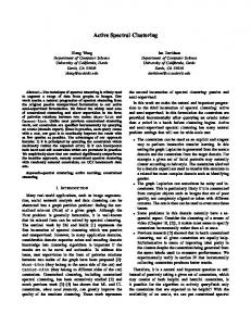
Figure 1: Two interlocked ring clusters: scatter plot of the data (left), affinity matrix A computed with the Gaussian kernel (middle) and the conductivity matrix C. 2003). Determining the kernel parameter σ is a pivotal issue and greatly influences on the final clustering result. In some cases the “right” σ is “obvious”. However, generally it is non-trivial to find a good σ value. A possible method is trying different values for σ and choosing the one which optimizes some quality measure (Ng et al., 2002). In contrast to many authors who focus their analysis on spectral properties, we believe that the crucial issue is the construction of a good affinity matrix which is as block diagonal as possible. In that case spectral decomposition is merely the most convenient way to discover this block structure. In order to amplify the block structure of an affinity matrix, we introduce the conductivity method, which is described in Section 2. This allows us to start with a weak affinity matrix where the affinities of many points might be close to zero. A context dependent way of constructing such weak affinity matrices is suggested in section 3. For the final clustering of the spectral images, we propose a novel algorithm, termed K-lines (Section 4). Section 5 compares our clustering method to other algorithms. We conclude with a discussion on the scope and limitations of the proposed methods (Section 6).

2

Block Structure Amplification

¡ ¢ Consider a block-diagonal affinity matrix A = 10 01 , where each 1 denotes an arbitrary-sized block of ones. The remaining zeros in the matrix are denoted by 0s. This block structure is easily discovered, e.g. by looking at the two dominant eigenvectors, i.e. the eigenvectors corresponding to the two dominant eigenvalues, of A. If the blocks are of different sizes, then the space spanned by eigenvectors is not rotation invariant. In that case, even the first eigenvector is sufficient for identifying the blocks. Furthermore, permutation of points does not make an essential difference, this only leads to a permutation of rows and columns of the matrix. The eigenvectors will be permuted respectively and the eigenvalues will remain unchanged. Therefore we also consider matrices to be block-diagonal if they are block-diagonal after a permutation of their rows and columns. An affinity matrix generated from real-world data is virtually never block-diagonal. If the clusters are nicely shaped (e.g. Gaussian) and well-separated, then the affinity matrix may be approximately block diagonal. For brevity, we will also refer to such matrices as block-diagonal. In contrast, consider the data set in Figure 1. Although the two rings are interlocked (like two links in a chain) and therefore not separated in a Euclidean sense, we tend to regard them as two distinct clusters. In this setting, the clustering intuition relies on continuous concentration of data points, a notion which was applied by (Ben-Hur et al., 2001). Two points belong to a cluster if they are close to each other, or if they are well connected by paths of short “hops” over the other points. The more such paths exist, the higher the chances are that the points belong to the same cluster. However, it is not immediately clear in this case how to obtain a good affinity matrix for clustering. Suppose a Gaussian kernel is used, then a large σ merges the clusters, resulting in an undesirable clustering. Choosing

Technical Report No. IDSIA-03-05

3

a small σ leads to a matrix which is approximately composed of two band-diagonal matrices. We will denote such matrices block-band. According to theoretical results using matrix perturbation theory (Ng et al., 2002) and empirical evidence (Section 5), spectral clustering can produce satisfactory results when the matrix is block-diagonal. For blockband matrices, the case is less clear from the theoretical point of view. The δ of the eigengap condition presented in (Ng et al., 2002) tends to zero when increasing the size of the sample, yet maintaining the same fixed band structure. As a consequence, the theory cannot guarantee a good solution. Simulations suggest that in practice the spectral clustering of a block-band matrix is good. However, the choice of σ in this case is significantly more difficult than for block-diagonal matrices. We must set σ small enough to obtain a weak affinity matrix, i.e. where only the affinities of directly neighboring points are high. On the other hand, σ must not be too small. Therefore, in some cases, the range of admissible σ’s can be very narrow. These considerations motivate a change of the affinity measure. Specifically, we want to amplify weak affinities in matrix A. Instead of considering two points similar if they are connected by a high-weight edge in the graph, we assign them a high affinity if the overall graph conductivity between them is high. We define conductivity as for electrical networks, i.e. the conductivity of two points depends on all paths between them. This measure should not be confused with the graph “conductance” by (Sinclair & Jerrum, 1989), which is – up to a constant factor – equivalent to the normalized cuts (Shi & Malik, 2000). In the normalized cuts approach, the overall flow between two disjunct graph parts is considered. Our approach is, in a sense, complementary: we consider the flow between any two points, and construct a new graph based on it. The conductivity for any two points xi and xj is computed in the following way. We first solve the system of linear equations: G · ϕ = ηij (1) where G is a N × N matrix constructed from the original affinity matrix A:  ½ 1 if q = 1   if p = 1 :  ½ 0P else G(p, q) =  k6=p A(p, k) if p = q  else :  −A(p, q) else

(2)

and ηij is an indicator vector of length N . It represents points xi and xj for which we want to compute the conductivity, and is composed as follows:   −1 for k = i and i > 1 1 for k = j ηij (k) = (3)  0 otherwise Solving Equation 1 gives us vector ϕ. The conductivity between xi and xj , i < j is then given by C(i, j) = 1/ [ϕ(j) − ϕ(i)] which, due to the fact that ηij is extremely sparse, can be simplified to £ ¤ C(i, j) = 1/ G−1 (i, i) + G−1 (j, j) − G−1 (i, j) − G−1 (j, i)

(4)

(5)

so that ηij never explicitly appears. Due to the symmetry, it follows that C(i, j) = C(j, i). The diagonal elements C(i, i) can be set to maxi,j C(i, j). It therefore suffices to compute G−1 only once, in O(N 3 ) time, and to compute the conductivity matrix C in O(N 2 ) time. An intuitive motivation for the above method comes from electrical engineering, where the method is known as node analysis. We consider a resistor network, where direct conductivities (i.e. inverse resistances) between two nodes i and j are denoted by Gij . To compute the overall conductivity between the nodes, we measure the voltage Uij between them when we let a known current I enter the network at node i and leave it at the node j. The overall conductivity is then given by Ohm’s law: Gij = I/Uij . The voltage is defined as the potential difference between the nodes: Uij = ϕj − ϕi , and the potentials can be computed from

Technical Report No. IDSIA-03-05

4

3

1

1

2

0.8 0.6 0.4 0.2 0 −0.2 −0.4 −0.6 −0.8 −1 2 1.5

1 1

0.5

0.5

0

0

−0.5

−0.5 −1

−1

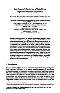
Figure 2: Two interlocked ring clusters with σ = 0.2

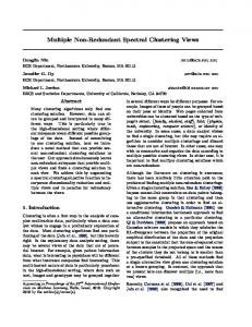
Figure 3: Two rings with low dispersion and a Gaussian cluster with large dispersion

P Kirchhoff’s law, stating that all currents entering a node i must also leave it: j6=i Iij = 0. Applying Ohm’s law again, the currents can be expressed over voltages and conductivities, so that this Equation becomes: P P G (ϕ − ϕ ) = 0. Grouping the direct conductivities by the corresponding potentials and G U = ij j i ij ij j6=i j6=i formulating the equation for all nodes, we obtain the Equation (1). The vector η represents the known current I, which we have transferred to the right side of the equation. As we know from graph theory, the adjacency matrix of a connected graph with N nodes is of rank N − 1. In our case that means that, if we would compose G relying only on Kirchhoff’s and Ohm’s law, its rows would sum to zero. In other words the system would be undetermined. In a physical sense, currents entering and leaving N − 1 nodes determine also the currents in the N -th node, since they have nowhere else to go. In order to obtain a determined system, we have to choose a node and fix it to a known potential, so it becomes the reference node. In our method we set the potential of the first node to zero (ϕ(1) = 0), which is reflected by the way the first rows of G and i are defined in Equations (2) and (3). ¡ ¢ The method here seems to require using a different ηij and solving the equations anew for all N2 pairs of nodes. That would be the computational analogy of connecting the current source between every pair of nodes and measuring the voltage. This, fortunately, is not the case: First, since direct conductivities between nodes do not change, it suffices to invert the matrix G only once. And second, for computing the overall conductivity between two nodes, we do not need all voltages in the network; the voltage between these nodes suffices. This allows us to observe only two rows in the G−1 matrix. Furthermore, the fact that for each vector ηij , all except two components are zeros (i.e. the external current source is attached only to two nodes), entails that we only need to consider two columns in G−1 . Consequently, the conductivity between any two nodes can be computed from only four elements of the matrix G−1 , as Equation (5) shows. The resulting conductivity matrix C is obtained from the matrix A, but displays a reinforced block structure. We may use C for the remainder of the spectral clustering task. But, before we proceed with it, we need to know how to construct A. Observe that (2) almost is the Laplacian of A, except for the first row. The first row may be regarded as a “trick” to make the matrix invertible. Thus, we gave a different motivation for using the Laplacian. In this light, observe the high similarity of our algorithm to that of Saerens et al. (2004). They consider a random walk criterion on the graph. Thus they arrive at a formula which is almost identical to (5), except for the inverse which is replaced by the pseudo-inverse of the Laplacian.

3

Constructing Affinity Matrices

In this section we consider the question of how to construct affinity matrices A, in¡ particular weak ones. We ¢ 2 restrict our discussion to the case that the affinities are Gaussian: A(i, j) = exp −kxi − xj k2 /2σij , where kxi − xj k denotes the Euclidean distance between xi and xj . Often, σ is set to a global value (σij ≡ σ). In this

Technical Report No. IDSIA-03-05

5

case the performance of spectral clustering depends heavily on the selection of σ. A common selection method is to try different values for σ and use the best one. This process can be automated in an unsupervised way as suggested by (Ng et al., 2002), since concentration of the spectral images may be an indicator for the quality of the choice of σ. Another possibility is to make use of the distance histogram. If the data form clusters, then we expect the histogram of their distances to be multi-modal. The first mode would correspond to the average intra-cluster distance and others to between-cluster distances. By choosing σ around the first mode, the affinity values of points forming a cluster can be expected to be significantly larger than others. Consequently, the affinity matrix is likely to resemble a block diagonal matrix. For a weaker affinity matrix, σ may and should be chosen smaller, below the first histogram mode. This is the case when using the conductivity method, which itself amplifies the weak affinities. We have found out empirically that, for this method, a good choice is at about half the position of the first peak in the distance histogram, or somewhat below. This distance histogram heuristic has the drawback that it cannot be automated in a robust way. Moreover, for some data sets, finding a single value of σ that performs equally well over the whole data set might not be even possible. Consider the two concentric rings and a Gaussian cluster in Figure 3. The points in the third, Gaussian cluster have a significantly larger dispersion than the points in the two rings. So each of the points in the third cluster will be connected to almost no other point than itself if σ is chosen correctly for the rings. However, a human would probably apply a context-dependent affinity in this case. For example, the affinity of the points labelled 1 and 2 should be higher than the affinity of points 1 and 3, although the latter distance is smaller. We therefore propose to use a context-dependent method for constructing the affinity matrix, rather than using a single σ for all points. For each point xi we suggest σi . This results in an ¢ ¡ to choose a different ˜ j) = exp −kxi − xj k2 /2σ 2 . In order to determine each asymmetric similarity matrix, which is given by A(i, i σi , we enforce the following condition: n X

¡ kxi − xj k2 ¢ exp − =τ 2σi2 j=1

(6)

for each 1 ≤ i ≤ n, where τ > 0 is a constant. That is, we choose σi such that the row sum of A assumes the fixed value τ . We may interpret τ as the fixed neighborhood size. Choosing τ is easier than choosing σ, since τ is scale invariant. We will see in Section 5 that, in contrast to σ, the clustering result is not very sensitive to the value of τ . In order to obtain weak affinities, τ is set to a small value, such that only immediately neighboring points obtain a significant affinity. We suggest the choice of τ = 1 + 2D, where D is the dimension of the data — there should be two neighbors for each dimension, plus one because the point is neighbor of itself. This value has been used for all simulations below. Now we can determine σi which satisfies Equation (6) by iterative bisection. Few iterations are sufficient, since there is no great precision required. In order to proceed with the conductivity matrix, we need to obtain a symmetric matrix A from the ˜ Again for a weak affinity matrix, high values should only exist between immediately asymmetric matrix A. neighboring points. Thus the affinity between xi and xj should be the smaller of the respective values, A(i, j) = ˜ j), A(j, ˜ i)}. This ensures that, for example, the points 1 and 3 in Figure 3 obtain a lower affinity value min{A(i, than the points 1 and 2. This is because point 1, although being nearer to point 3, actually lies in the relative neighborhood of point 2. The idea to consider a context-dependent neighborhood is not new. A very interesting parallel approach is given by Rosales and Frey (2003). While they suggest and motivate an EM-like repeated update of the neighborhood size, our method is heuristic and computationally cheaper. Compare also the row normalization by Meil˘a and Shi (2001). Very recently, Zelnik-Manor and Perona (2004) have suggested another local neighborhood approach which is very similar to ours.

4

Clustering the Spectral Images

Given the conductivity matrix C (or the affinity matrix A, if conductivity is not applied), we compute the £ ¤ matrix of the dominant eigenvectors V = v1 . . . vK ∈ RN ×K , that is the eigenvectors which correspond to

Technical Report No. IDSIA-03-05 Name 2R3D.1 2R3D.2 2RG 2S 4G 5G 2Spi Iris Wine BC

N 600 600 290 220 200 250 386 150 178 683

K 2 2 3 2 4 5 2 3 3 2

D 3 3 2 2 3 4 2 4 13 9

197 195 110 26 24 41 191 16 5 26

K-means (197.9 ± 1.0) (195.1 ± 0.2) (125.3 ± 2.4) (34.5 ± 6.4) (40.0 ± 24.2) (62.0 ± 27.8) (192.3 ± 0.5) (27.8 ± 22.2) (8.7 ± 10.5) (26.5 ± 0.5)

6

0 68 66 25 2 13 151 8 3 20

Girolami (162.2 ± 86.4) (202.9 ± 54.6) (121.7 ± 26.5) ( 49.9 ± 26.6) ( 2.6 ± 5.8) ( 21.2 ± 14.1) (178.5 ± 10.7) ( 10.3 ± 2.2) ( 3.9 ± 0.9) ( 21.5 ± 1.0)

0 4 101 0 18 33 0 14 3 22

Ng et al. ( 17.7 ± 70.4) ( 7.5 ± 28.9) (102.2 ± 3.8) ( 9.3 ± 10.8) ( 35.1 ± 22.2) ( 40.1 ± 14.6) ( 79.1 ± 95.4) ( 14.8 ± 3.6) ( 3.3 ± 0.5) ( 22.8 ± 0.6)

0 6 2 97 2 13 0 10 12 21

Our-σ (0.0 ± 0.0) (8.2 ± 1.9) (16.8 ± 38.0) (101.8 ± 4.8) (3.0 ± 7.0) (34.5 ± 14.6) (39.4 ± 55.5) (12.3 ± 5.3) (18.9 ± 6.6) (25.1 ± 2.0)

Our-τ 0 93 0 0 1 11 193 7 65 20

Table 1: Empirical comparison of the algorithms for different data sets. N denotes the number of points in the set, K the number of clusters, and D the data dimensionality. For each algorithm we document the minimum number of incorrectly clustered points and the mean and standard deviation (due to using a different σ in each run) in brackets. The respective best value is bold. We present two variants of our algorithm: “Our-σ” denotes the algorithm with a global kernel width determined from the distance histogram. “Our-τ ” denotes the algorithm with a point-specific σi , according to Eq. 6. £ ¤ the K largest eigenvalues. Then we call y1 . . . yN = Y = V 0 ∈ RK×N the spectral images of the original data x1 , . . . , xN . There are different ways to compute the final clustering from the spectral images y1 , . . . , yN . The images of points belonging to the same cluster were experimentaly observed to be distributed angularly around straight lines — the more compact the cluster, the better alignment of the spectral images. A simple, off-the-shelf clustering algorithms like K-means cannot be used, because it assumes approximately round clusters. To circumvent the problem, (Ng et al.) suggest projecting the points on the unit sphere and then using K-means. However, this leads to a certain loss of information (namely the radius), and the resulting clusters are still not round. We propose a similar algorithm here, which exploits the observed structure of the clusters and which we have found to be slightly superior in the simulations (compare a parallel approach, the K-planes algorithm in (Bradley & Mangasarian, 2000)). Algorithm K-lines Each cluster is given by a line through the origin, represented by a vector mi ∈ Rk of unit length, 1 ≤ i ≤ k. 1 Initialize m1 ...mK (e.g. by the canonical unit vectors) 2 For each i ∈ {1, . . . , k}, let Si be the set of points containing all points yj that are closest to the line defined by mi 3 For each i ∈ {1, . . . , k}, let mi define the line through the origin which has smallest sum square distance to all points in Si 4 Repeat from 2 until convergence Our final spectral clustering algorithm then reads as follows. Algorithm Context dependent clustering with block amplification ˜ and A. 1 Calculate the context dependent affinity matrices A 2 Construct the conductivity matrix C according to (5). 3 Determine K principal eigenvectors, e.g. by Lanczo’s method, and compute the spectral images y1 , . . . , yn . 4 Cluster y1 , . . . , yn by K-lines.

5

Simulations

We present simulation results and compare our proposed method with three other clustering algorithms: standard K-means, a more sophisticated, kernel-based expectation-maximization method (Girolami, 2002), and the algorithm suggested by (Ng et al.). Whereas K-means simply assumes K spherical clusters and looks for their centers, the (Girolami) method projects the data into a feature space and clusters them there using a standard EM method. The (Ng et al.) algorithm differs from ours in the way it computes and scales the affinity matrix,

Technical Report No. IDSIA-03-05

7

4G

2S

2Spi

2 1 0 1

1

0

0 −1 −1

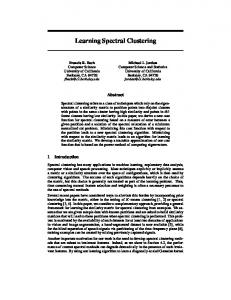
Figure 4: Data sets, left-to-right: 2S, 4G, and 2Spi. and by using K-means instead of K-lines in the final step. All algorithms are evaluated on a number of benchmark and real-world data sets. Assessing the quality of a clustering algorithm is not easy. First, clustering is an ill-posed problem. We overcome this difficulty by defining an “optimal” reference clustering: For the artificial data sets, we know the probability distribution which generated the data, whereas for the real world data sets labels are available which we use for reference (but which are unknown to the clustering algorithm). Another problem is that the outcome is partly very sensitive to the choice of the kernel parameter σ. In order to give a somewhat realistic evaluation of the (Girolami) and the (Ng et al.) algorithms which depend on this parameter, the experiments were performed in two phases: First, for each data set we systematically scanned a wide range of σ’s (the range was set manually to cover most of the distance histogram) and ran the clustering algorithms. We denote by σ ∗ the σ which produced the best results. In the second phase, we performed 100 runs, with σ randomly sampled form [σ ∗ ± 20%]. The rationale for this procedure is that the optimal σ cannot be known in real-world application, but the experimenter will probably be able to guess it with some precision (which we suppose to be somewhere around ±20%) based on the distance histogram. The automatic computation of σ, as suggested by (Ng et al., 2002), sometimes led to suboptimal σ and, consequently, to poor results. In most cases, the histogram method resulted to a σ very close to the best value and led to very similar results. We present the best result found as well as the mean and standard deviation. In contrast, our context-dependent algorithm produced deterministic results, because K-lines was initialized deterministically, and the neighborhood size was set to τ = 2D + 1, where D is the dimension of the data. Therefore, for this algorithm we refrain from quoting the mean and standard deviation. The experimental results are summarized in Table 1. The data set 2R3D.1 was presented in Figure 1 as a motivation for conductivity. It is an artificial data set, obtained by dispersing points around two interlocked rings in 3D. The dispersion is Gaussian, with standard deviation equal to 0.1. This set is impossible to cluster by K-means, but other algorithms have no problem with it. Conductivity-based algorithm (Our-σ) is, however, more stable than competing algorithms. 2R3D.2 is similar, but with the double standard deviation of the points around the rings. Here, all algorithms start having problems. Although Ng et al algorithm is the best considering the number of false assignments, it is less stable than the conductivity method. The context-dependent approach is of no advantage here and is clearly outperformed, since the dispersion of points in clusters is constant. The ring segments passing through the center of the other ring are incorrectly assigned to that ring. Our interpretation is that the context-sensitive kernel width acts as a drawback in this situation, since it actually abolishes the already weak gap between the clusters. The next four data sets have varying data dispersions and thus the context-dependent approach is clearly superior. 2RG is the data set from Figure 3, 2S consists of two S-shaped clusters with inhomogeneous dispersion in 2D, and 4G and 5G have four and five Gaussian clusters with different dispersion in 3D and 4D, respectively.

Technical Report No. IDSIA-03-05

8

Due to the different dispersions of clusters and, in the case of 2S within clusters, no obvious global σ can be chosen. 2Spi is a variant of Wieland’s two spirals (see Fahlman, 1988) with double point density (193 points per spiral). Contrary to our expectations this is one of the examples where the context-dependent approach fails; it is only successful on the fourfold density problem. The last three data sets are common benchmark sets with real-world data (Murphy & Aha, 1994): the iris, the wine and the breast cancer data set. Both our methods perform very well on iris and breast cancer. However, the wine data set is too sparse for context-dependent method: only 178 points in 13 dimensions, giving the conductivity too many degrees of freedom to connect the points. If the context-dependent method is used without the conductivity, then the algorithm also achieves a good clustering, with only four false assignments. Our algorithm yields good results on most of the data sets. In addition, it is very insensitive to the choice of the neighborhood size τ . For example, all results remain the same if the constant value τ = 10 is used instead of τ = 2D + 1. The Ng et al. algorithm also produces very good experimental results, if σ is well chosen. However, the range of good values for σ may be very small. It this case, conductivity can significantly improve robustness. For the data sets 2R3D.2 and 2Spi for example, a symmetric algorithm which uses conductivity displays a variance much lower than for the Ng et al. algorithm (Table 1). The increased robustness of the conductivity method can also be observed in the computation time required for the spectral decomposition (with the implementation of Lanczo’s method coming with MATLAB). Computing the spectrum of the conductivity matrix needs only about 70% of the time which is needed for computing a block-band matrix. Finally, we note that our context-dependent way of constructing affinities can handle data which is inhomogeneously distributed. It works well if data is sufficiently dense and tends to fail if the data is too sparse.

6

Conclusions

Amplifying the block structure of the affinity matrix can improve spectral clustering. This method allows us to start with a weak affinity matrix, where only immediately neighboring points have significant affinities. The conductivity method yields a matrix which is relatively close to block diagonal. Such matrix may be used for clustering with spectral methods. For constructing a weak affinity matrix, we have proposed a contextdependent method which is easily automated and not sensitive to its parameter, the neighborhood size τ . This affinity measure compares favorably with the Gaussian kernel. For the clustering of the spectral images, we have proposed the K-lines algorithm. The resulting spectral clustering algorithm is fully automatic and very robust, and it displays good performance in many cases. It tends to fail on sparse data. All three methods we proposed – conductivity, context-dependent affinity, and K-lines – can be used independently from each other as components in (spectral) clustering algorithms. We have motivated our methods by purely intuitive and empirical means; a theoretical justification remains open. Future issues to investigate would be: (a) Study the properties of the conductivity matrix with respect to graph partitioning criteria. (b) Give quantitative assertions on the spectrum of the conductivity matrix. (c) Find out more about the distribution of the spectral images, thus giving a sound foundation of K-lines or another method. Authors generally agree that it is still incompletely understood how and why spectral clustering works. However, this might be the wrong question to pose. Spectral decomposition might be only one convenient way to discover the block structure of the affinity matrix, there may be other ways to achieve this. In our opinion, the central issue is constructing a “good” affinity matrix from the data with a block structure as expressed as possible.

7

Acknowledgements

We would like to thank Efrat Egozi, Michael Fink, Yair Weiss, and Andreas Zell, for helpful suggestions and discussions. Igor Fischer is supported by a Minerva fellowship, and Jan Poland by BMBF grant 01 1B 805 A/1 and by SNF grant 2100-6712.02.

Technical Report No. IDSIA-03-05

9

References Alpert, C., Kahng, A., & Yao, S. (1994). Spectral partitioning: The more eigenvectors, the better (Technical Report). UCLA CS Dept. Technical Report #940036. Ben-Hur, A., D. Horn, H. S., & Vapnik, V. (2001). Support vector clustering. Journal of Machine Learning Research, 2, 125–137. Bradley, P. S., & Mangasarian, O. L. (2000). k-plane clustering. Journal of Global Optimization, 16, 23–32. Fahlman, S. (1988). Faster-learning variations on back-propagation: An empirical study. Proceedings of the 1988 Connectionist Models Summer School (pp. 38–51). San Mateo, CA, USA: Morgan Kaufmann. Girolami, M. (2002). Mercer kernel-based clustering in feature space. IEEE Transactions on Neural Networks, 13, 780–784. Kannan, R., Vempala, S., & Vetta, A. (2000). On clusterings: Good, bad and spectral. Proceedings of the 41st Symposium on Foundations of Computer Science. Meil˘a, M., & Shi, J. (2001). Learning segmentation by random walks. Advances in Neural Information Processing Systems 13 (pp. 873–879). MIT Press. Murphy, P., & Aha, D. (1994). UCI repository of machine learning databases. Ng, A., Jordan, M., & Weiss, Y. (2002). On spectral clustering: Analysis and an algorithm. Advances in Neural Information Processing Systems 14. Cambridge, MA: MIT Press. Perona, P., & Freeman, W. (1998). A factorization approach to grouping. Lecture Notes in Computer Science, 1406, 655–670. Rosales, R., & Frey, B. (2003). Learning generative models of affinity matrices. 19th Conference on Uncertainty in Artificial Intelligence (UAI). Saerens, M., Fouss, F., Yen, L., & Dupont, P. (2004). The principal component analysis of a graph, and its relationship to spectral clustering. Proceedings of the 15th European Conference on Machine Learning (ECML 2004) (pp. 371–383). Springer. Shi, J., & Malik, J. (2000). Normalized cuts and image segmentation. IEEE Transactions on Pattern Analysis and Machine Intelligence, 22, 888–905. Sinclair, A., & Jerrum, M. (1989). Approximate counting, uniform generation and rapidly mixing markov chains. Information and Computation, 82, 93–133. Spielman, D. A., & Teng, S. (1996). Spectral partitioning works: Planar graphs and finite element meshes. IEEE Symposium on Foundations of Computer Science (pp. 96–105). Verma, D., & Meil˘a, M. (2003). A comparison of spectral clustering algorithms (Technical Report). UW CSE. Technical report 03-05-01. von Luxburg, U., Boudquet, O., & Belkin, M. (2004). Towards convergence of spectral clustering on random samples. COLT (pp. 457–471). Weiss, Y. (1999). Segmentation using eigenvectors: A unifying view. ICCV (2) (pp. 975–982). Zelnik-Manor, L., & Perona, P. (2004). Self-tuning spectral clustering. NIPS 2004, to appear.