An Accurate and Efficient Algorithm for Parameter ...

International Journal of Applied Physics and Mathematics, Vol. 1, No. 2, September 2011

An Accurate and Efficient Algorithm for Parameter Estimation of 2D Acoustic Wave Equation Wenyuan Liao 

of fact, the complete mathematical solution of this questions is quite complicated, and is still partially answered or even unanswered at all. One difficulty in solving an inverse problem is the instability, which means that a set of almost perfect observational data could produce a totally wrong result. Although the problem is still not solved completely, some important progresses on the stability were made in the past. According to Isakov, the inverse problem is stable if some smooth conditions for the domain, initial and boundary conditions are satisfied. More details regarding the well-posedness of the inverse problem can be found in [8]. For homogeneous wave equation, the analytical solution can be obtained for certain initial and boundary conditions. However, for the general case, the analytical solution is difficult to get, thus we should use numerical methods to solve the forward problem when an inverse problem is solved. In this paper, we applied a second-order accurate central finite difference approximation for time derivative and a fourth-order finite difference schemes to approximate u xx and u yy .

Abstract—An efficient and accurate numerical method has been proposed in this paper to estimate the acoustic coefficient in a 2D acoustic wave equation. The inverse problem is formulated as a PDE-constrained optimization problem, in which the forward problem is numerically solved by both efficient finite difference schemes. To generate the gradient of the quadratic misfit function with respect to the unknown coefficient, the widely used automatic differentiation tool TAMC is used. Finally a gradient-based optimization algorithm is applied to minimize the misfit function. Numerical results are presented to show that the proposed method is effective and robust in estimating the acoustic coefficient. Index Terms—Inverse problem; wave equation; finite difference method; adjoint method; optimization.

I. INTRODUCTION The identification of model coefficients in an acoustic wave equation through observational data plays a crucial role in applied mathematics, geo-science, physics and many other areas. This technique has been widely used to determine the unknown property of a medium in which the wave is propagated by measuring data on its boundary or a specified location in the domain. A great deal of work have been done and many direct and indirect methods have been reported in the past decades [1-4,10]. In the wave equation, the unknown coefficient which characterizes the property of the medium is important to the physical process but usually cannot be measured directly, or very expensive to be measured, thus some mathematical method is needed to estimate it. In this paper, we extend the method developed in [5] to a 2D acoustic wave equation subject to extra boundary condition. The wave equation has been widely used in modeling wave propagation in mediums such as earth. It is quite often that geophysicists need to know the internal structure of a certain area of the earth. However, due to the high drilling cost, it is impossible to drill many wells and examine the rock samples. Fortunately, the underlying mathematical model that describes the wave propagation is well understood, and it is much easier and more cost-effective to record the wave information on the surface of the domain of interest. Such technique forms exactly an inverse problem of wave equation. The basic question is: is it possible to recover the coefficient from the measurements on the surface of the interested part of the earth? As one can expect, there is no simple answer for this question, as a matter

An accurate gradient is critical in minimizing the cost functional. Herein we apply automatic differentiation tool TAMC to generate discrete adjoint, then use it to calculate the gradient. The rest of this paper is organized as the following. In section 2, we formulate the inverse problem as a PDE-constrained optimization problem, followed by the description of an efficient finite difference scheme to solve the wave equation. In section 4 the automatic differentiation tool TAMC is briefly introduced, while the optimization package is introduced in section 5. Some numerical results are presented in section 6 and finally some conclusions are addressed.

II. MATHEMATICAL FORMULATION OF THE INVERSE PROBLEM Let us consider the following 2D wave equation u tt  c ( x , y )( u xx  u

yy

)  S (x, y,t)

(1)

satisfying the initial and boundary conditions: u ( x , y ,0 ) = u 0 ( x , y ), ( x , y ) ∈ Ω u t ( x , y , 0 ) = u 1 ( x , y ), ( x , y ) ∈ Ω u ( x , y , t ) = φ ( x , y , t ), ( x , y , t ) ∈ Ω × ( 0 , T )

(2) (3) (4)

and subject to the extra boundary condition:  u /  n   ( x , y , t ), ( x , y , t )     ( 0 , t )

(5) where c( x, y ) is the unknown acoustic coefficient, n is the outer normal orientation of  , u0 (x, y), u1 ( x, y), (x, y, t) and (x, y, t) are functions that satisfy some regularity conditions,  is the boundary of the square domain  . For the sake of simplicity, throughout this paper, we assume that

Manuscript received July 12, 2011; revised August 10, 2011. Wenyuan Liao,Department of Mathematics and Statistics, University of Calgary Calgary, Alberta, T2N 1N4, Canada (E-mail: [email protected])

96

International Journal of Applied Physics and Mathematics, Vol. 1, No. 2, September 2011   [ 0 , L ]  [ 0 , L ] , with L be a positive constant.

approximate u xx and u yy with only second-order accuracy, where  x2 / h 2 and  y2 / h 2 are defined as:

If the coefficient is known, the problem (1)-(5) is obviously over-specified because of the extra boundary condition in (5). However, since the coefficient c( x, y ) is unknown, a unique solution may exist and can be obtained through solving an inverse problem governed by the wave equation. Here we assume that the initial and boundary conditions are sufficiently smooth to guarantee a unique solution. More details regarding the existence and uniqueness can be found in [8,18]. The numerical procedure to estimate c( x, y ) and corresponding solution u(x, y, t) is inherently an iterative procedure, which includes three main steps: 1. Starting from an initial guess c 0 ( x, y) , the forward problem defined in (1)-(4) is solved. 2. The numerical result from step 1 is compared with the condition in Eq. (5) to calculate the cost functional, then the gradient (derivative) of the cost functional with respect to c 0 ( x, y) is calculated from the adjoint. c ( x, y )

2

+ μ ∇ c( x, y )

2

 u i , j  u i , j 1  2 u i , j  u i , j 1 ,

(8)

In order to obtain fourth-order approximation in space, we replace  x and  y by  x (1   x2 / 12 ) and  y (1   y / 12 ) respectively. Based on the approximation, the original wave equation in (1) is transformed to the following ODE system 2

2

(u

i, j

) tt 

2

c i, j   h 2 

2 x

2

 

2 y





4 x

  12

4 y

 u  

i, j

2

 s i, j (t )

(9)

with ci, j  c(xi , y j ),ui, j (t)  u(xi , y j , t) , si, j (t)  s(xi , yj ,t). Depending on the discretization of time derivative, the numerical methods for the ODE system (9) can be classified into two categories: explicit and implicit schemes. The explicit scheme is efficient but only conditionally stable, so in general small time step size is required. The implicit scheme is usually unconditionally stable but a linear or nonlinear algebraic system needs to be solved at each time step, which makes it less efficient. A detailed comparison can be found in [6,7]. In this paper, we apply the central finite difference scheme to the second-order time derivative, and obtain the following formula:

+

2 T ∂ u~ ( c ( x , y ); x , y , t ) ⎞ ⎛ ⎟ dsdt ∫0 ∂∫Ω⎜⎝ ϕ ( x , y , t ) − ∂n ⎠

(7)

2 y

3. Optimization algorithm is applied to minimize the cost functional, and the three steps are repeated till convergence is obtained. Here the cost functional J(c(x, y))is defined as J ( c ( x , y )) = λ c ( x , y )

 x2 u i , j  u i  1 , j  2 u i , j  u i  1 , j ,

u ik, j 1  2 u ik, j  u ik, j 1 t 2

(6)



 4   y4 c i, j  2   x   y2  x 12 h 2 

 u i , j  s i , j (t )  

(10)

which is second-order accurate in time and fourth-order accurate in space. Note that two initial conditions are needed in (10) but only u0 ( x, y) is given explicitly in (2), so we

where u~ ( c ( x , y ), x , y , t ) is the solution of the initial-boundary value problem (1-4) based on c( x, y ) , ds is the line integral along the boundary of  ,  and  are non-negative regularity parameters. Note that in real computation, the integral in (6) is implemented by some high-order numerical methods such as Simpson's formula. A detailed discussion on how to choose these parameters  and  to ensure the existence and uniqueness, and to improve the accuracy and efficiency of the solution is available in [5]. In general, if the user has no prior information regarding c( x, y ) , they can simply set the parameters as zeros, although it may cause the inverse problem be ill-posed.

need to find a second-order accurate approximation of the second initial condition. Namely we have  u i, j

2  t 2  u i, j t0 t t 2 2 2 t  u 0 ( x i , y j )   tu 1 ( x i , y j )  u 2 ( x i , y j ), 2

u i, j (  t )  u i, j (0 )   t

t0



(11)

where u2 ( xi , y j )  ci , j ((u0 ) xx  (u0 ) yy )i , j  s( xi , y j ,0) , and the truncation error of the approximation is t 3 . Once the numerical solution based on an initial guess c 0 ( x, y ) is available, we can use the observational data to calculate the cost functional. Since the extra boundary condition in Eq. (5) is Neumann boundary condition, the numerical solution cannot be used directly. We firstly apply Taylor expansion at the boundary points to approximate u / n . Since the numerical scheme for the forward problem is second-order in space, the interpolation scheme should be second-order accurate at least. For example, the following schemes can be used to approximate the boundary conditions:

III. FINITE DIFFERENCE METHOD FOR THE WAVE EQUATION For special initial and boundary conditions, the initial-boundary value problem defined in (1)-(4) can be solved analytically, but it becomes almost impossible when a general initial and boundary value problem is considered. Thus, accurate and efficient numerical schemes are needed to solve the wave equation. To simplify the discussion, we assume that the domain  is divided into a uniform N  N grid with step sizes h  h x  h y  L /( N  1 ) .For convenience, we also assume that time step size  t  T /( M  1) is used for time integration. The numerical solution of u(x, y, t) at grid point ( xi , y j ) and time level t k  kt is denoted as u ik, j . It is well-known that the central finite difference operators  x2 / h 2 and  y2 / h 2 97

u x

ttn x0

 (  3 u 1n, j  4 u 2n, j  u 3n, j ) /( 2  x ), j  1, 2 ,   N

u x

ttn xL

 ( u Nn  2 , j  4 u Nn  1 , j  3 u Nn , j ) /( 2  x ), j  1, 2 ,   N

u y

t t n y 0

 (3u in1,1  4u in, 2  u in,3 ) /(2y ), i  1,2,   N

u y

t t n yL

 (u in1, N  2  4u in, N  2  3u in, N ) /(2y ), i  1,2,  N

International Journal of Applied Physics and Mathematics, Vol. 1, No. 2, September 2011 n where ui , j is the numerical solution at the grid point ( xi , y j )

parameters. It is well-known that L-BFGS, which implements Quasi-Newton method, uses the BroydenFletcher-Goldfarb-Shanno update to approximate the Hessian matrix. Consequently, unlike the regular BFGS algorithm, the L-BFGS only maintains a very short history of the past updates, thus the requirement on storage has been reduced significantly. Let f(x) be the function to be minimized, g(x) be the gradient, and xk be the result of k-th iteration, we can define

n at time level t , based on the initial guess c0 ( x, y) . The time integral is implemented by Simpson’s rule, which is fourth-order accurate. So eventually the cost functional is a function of c( x, y ) .

IV. DISCRETE ADJOINT GENERATED BY AUTOMATIC DIFFERENTIATION

s k  x k 1 x k ... and

yk = gk +1 − gk , the L-BFGS method is defined as the following: Step 1: Set initial guess X0 and let K=0, choose parameter m, which is the number of BFGS corrections that are to be kept. Choose a sparse symmetric and positive definite matrix H0, which approximates the inverse Hessian matrix of f(x). Choose two parameters ~ and  as 0 < τ~ < 1 / 2 and ~    1. Step 2: Compute d k = − H k g k and x k +1 = x k + α k d k , where  k is a parameter satisfying the Wolf conditions:

The success of the gradient-based optimization relies on an accurate derivative of the cost functional with respect to the unknown coefficient. In this section we use TAMC to generate the discrete adjoint which will be used to calculate the gradient. In real computation, c( x, y ) has to be discretized on a finite grids thus we can only estimate it on a finite number of grid points, although theoretically it can be a continuous function in some function space. Here we assume that c( x, y ) is estimated on the same grid as that on which the wave equation is solved. If the size of the unknown coefficient is small, one can use finite difference quotient, which is a simple technique to calculate the gradient. However when the size of the unknown parameters increases, this method becomes too expensive to be practical. The adjoint method has been widely used to calculate the gradient for large-size problem. In principle both continuous and discrete adjoint methods can be used to derive the gradient. Theoretically, there is no formal advantage of one method over another one in any general sense, however one method may be better suited to a given application. In the method of continuous adjoint, the adjoint equation, which is derived using methods such as calculus of variations, is numerically solved to generate the gradient. While in the method of discrete adjoint, the numerical scheme for the direct problem defined in (1)-(4) is considered as the forward model, thus this approach actually computes the derivatives of the numerical solution, rather than approximating the derivatives of the exact solution. To derive the discrete adjoint, one can either take the adjoint of the forward numerical scheme directly, or apply automatic differentiation tool such as TAMC [11-13]. Since the direct approach is time-consuming and error-prone, the automatic differentiation, which builds a new augmented program based on the program to solve the forward problem, had been widely used. Another advantage of automatic differentiation is its quick and simple implementation, since the user just needs to provide a numerical program to calculate the cost functional and the automatic differentiation tool will generate an adjoint program which will compute the gradient.

f ( xk + α k d k ) ≤ f ( xk ) + τ~α k g kT d k and

g ( xk + α k d k )T d k ≥ τg kT d k . Step 3: Let m min{k,m 1}, and update the matrix

m  1 times using the pairs

{ y j , s j }kj  k  m

Hk

and the

following formula:  V k  I  y k s kT /( y kT s k )   T T T H  k  1  V k H k V k  s k s k /( y k s k ) Step 4: Set k = k + 1 and go to Step 2. A detailed description of the algorithm can be found in [15,16]. It has been shown [17] that this package is very robust and converges faster than many other popular methods such as the widely used standard conjugate gradient method. For comparison, we also tested three conjugate gradient optimization algorithms: the Fletcher-Reeves method, the Polak-Ribiere method and the Positive Polak-Ribiere method. Conjugate gradient method has been widely used to solve nonlinear optimization problem. Again suppose f (x) smooth function to be minimized, and g (x) is its gradient. Let x 0 be the initial guess, g0 g(x0), and x k be the k-th iteration, the conjugate gradient method is implemented as the following: is a

 g k  dk     g k  b k d k 1 

k 0 k 1

x k 1  x k   k d k

where bk is a scalar and  k is a step length determined by means of a one-dimensional search. The three methods that are implemented in the package CG+[14] are almost identical with the only difference in the formula to calculate bk .

V. OPTIMIZATION ALGORITHMS We now provide a brief introduction to the optimization algorithm that will be used to solve the PDE-constrained optimization problem. L-BFGS, which stands for 'limited memory BFGS, will be used mainly because it is very efficient in solving optimization problem of large size

In the Fletcher-Reeves method, b k  g k / g k 1 , in the 2

2

Polak-Ribiere method, b k  g k , g k  g k 1 / g k 1 , while in 2

the positive Polak-Ribiere method, bk is calculated as 98

International Journal of Applied Physics and Mathematics, Vol. 1, No. 2, September 2011

b k  max{ g k , g k  g k 1 / g k 1 ,0} 2

square norms, which are defined as the following MAX  max c( xi , y j )  c~i , j

thus only non-negative bk is allowed in this method. It is worthy pointing out that the user can use any other gradient-based optimization algorithm to solve the optimization problem, since the proposed computational method is very flexible, and a new component can be easily integrated. Also the definition of the cost functional may affect the choice of the optimization algorithm as well. For more details, the readers are referred to the papers mentioned above.

1 i , j  N

RMS 

N



i , j 1

c( xi , y j )  c~i , j )2 / N 2

(12)

(13)

~ where ci , j is the estimated value of c( xi , y j ) .

VI. NUMERICAL RESULTS AND DISCUSSIONS We solve the initial-boundary value problem given in (1)-(5) defined on [0,1] × [0,1] and t  [0,1] . Here S(x, y,t) , initial and boundary conditions are chosen accordingly so that u(x, y,t) = e−t (sin(x) + cos(y)) and c( x, y)  1/(1  x2  y 2 ) . In this example, we set the two regularity parameters in (6) be zeros, as we assume that we have no prior information about c( x, y ) . We first validate the discrete adjoint generated by TAMC then illustrate the efficiency and accuracy of the proposed computational method. To validate the discrete adjoint generated by TAMC, we first calculate the finite difference quotient approximations of J / ci, j at several selected grid points with various values of  . The approximated derivatives are then compared with the results generated by TAMC at the same grid points. The numerical test is conducted on the grid with t 1/ 40 and hx hy 1/20 . Such grid is chosen to ensure the stability of the numerical method in (10), and that the numerical solution of the wave equation is accurate enough. Finally, the grid cannot be too fine otherwise the computational cost will be an issue. The results in Table I show that TAMC generates very accurate discrete adjoints. The first column contains the grid points where the adjoint is calculated, while column 2 to 4 contain the finite difference approximations of the adjoints by using various values of  . As we can see, when  is reduced from 0.1 to 0.001, the finite difference approximation converges to the results generated by TAMC, which is presented in column 5. Note that here we listed the results on 5 selected grid points only although it is possible to do so on all grid points, due to the space limit. However it is sufficient to show that TAMC is an effective and accurate tool to generate adjoint.

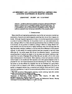
Fig. 1.Cost functional vs number of iterations

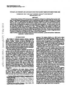
Fig. 2.Accuracy of the results vs number of iterations

TABLE I: COMPARISON OF DERIVATIVES BY VARIOUS METHODS

( xi , y j )

  0.1

  0.01

  0.001

TAMC

(0.1, 0.1) (0.2,0.2) (0.3, 0.3) (0.4,0.4) (0.5, 0.5) (0.6,0.6) (0.7, 0.7) (0.8,0.8) (0.9, 0.9)

-0.01536 -0.26358 -0.17491 -0.14826 -0.09188 -0.04497 -0.01437 -0.00129 0.00167

-0.01617 -0.27542 -0.18262 -0.15486 -0.09596 -0.04697 -0.01501 -0.00134 0.00122

-0.01613 -0.27667 -0.18343 -0.15555 -0.09639 -0.04718 -0.01508 -0.00135 0.00121

-0.01614 -0.27680 -0.18352 -0.15563 -0.09644 -0.04721 -0.01509 -0.00135 0.00121

Fig. 3.2D view of the difference

The result presented in Fig. 1 shows that the gradient generated by TAMC is accurate and effective, since the cost 8 functional reduces to zero rapidly(It is below 10 after 50 iterations). Consequently, the estimated c( x, y ) is also accurate as we can see from Fig. 2 that, both maximal and root mean square norms of the error are reduced to the level 3 of 10 after 50 iterations. Finally, to see how accurate the

As a measure of the accuracy of the computational method, we consider the difference in both maximal and root mean 99

International Journal of Applied Physics and Mathematics, Vol. 1, No. 2, September 2011

estimated c( x, y ) is, we plot the 2D view of the difference between the exact and estimated coefficient c( x, y ) in Fig. 3, which clearly demonstrates that the estimated coefficient is very accurate. To investigate the impact of the optimization algorithm on the result, we include the results by using L-BFGS and three Conjugate-Gradient algorithms: the Fletcher-Reeves (F-R) method, the Polak-Ribiere(P-R) method and the positive Polak-Ribiere (P P-R) method in the following table. The comparison is conducted when the RMS error for each case satisfies the specified tolerance, but the total number of function evaluations are different thus the total CPU time for each case varies significantly. Remark: The CPU time in Table 2. is the average of three runs.

method depends on various factors such as the numerical schemes for solving the forward problem, the method to generate the adjoint code, the choice of regularity parameters, the optimization algorithm used to minimize the cost functional, etc, and these issues will be further investigated in our future work. ACKNOWLEDGMENTS This work is supported by the Natural Sciences & Engineering Research Council of Canada (NSERC). REFERENCES [1]

TABLE II:PERFORMANCE COMPARISON AMONG VARIOUS ALGORITHMS RMS