and second-order accuracy for boundary mesh points. In our computer ... method on a two dimensional Luo-Rudy phase I action potential model. For a fixed ...
Proceedings of the 2006 WSEAS International Conference on Mathematical Biology and Ecology, Miami, Florida, USA, January 18-20, 2006 (pp81-86)
A Highly Efficient and Accurate Algorithm for Solving the Partial Differential Equation in Cardiac Tissue Models J ICHAO Z HAO1 , Y INBIN J IN2 , L I M A3 , ROBERT M. C ORLESS1 1
Department of Applied Mathematics University of Western Ontario London, Ontario, N6A 5B7, Canada
{jzhao29,rcorless}@uwo.ca 2
School of Life Science and Technology, 3 the First Hospital Xi’an Jiaotong University Xi’an, 710049, China
{ybjin,lma}@mail.xjtu.edu.cn Abstract:- We give a highly efficient, accurate and unconditionally stable algorithm to solve the partial differential equation for simulating the action potential propagation through cardiac tissue. In the new algorithm, we discretize the space domain by combining a compact finite difference scheme with an alternating direction implicit (ADI) scheme, which has fourth-order accuracy for interior mesh points, and second-order accuracy for boundary mesh points. In our computer simulation, we test the new method on a two dimensional Luo-Rudy phase I action potential model. For a fixed mesh grid N , the compact finite difference ADI method yields 50% more accuracy than the Crank-Nicolson ADI method. Furthermore, it costs almost the same amount of time as the Crank-Nicolson ADI method. On the other hand, if we want to obtain the same accuracy, it only costs 49% ∼ 65% of computational time if we use our compact finite difference ADI method instead of the Crank-Nicolson ADI method. Key-Words:- Compact finite difference method, ADI, Cardiac tissue models, Computer simulation, Spiral wave
1
Introduction
Cardiac tissue conduction models and computer simulation study have made the realization of the heart from qualitative analysis to quantitative analysis. These could be invaluable in the research of the foundation of cardiac arrhythmia and in the development of drugs for the treatment of various diseases caused by cardiac electric disorders. Until now there are two major classes of models of cardiac tissue: ionic models (Luo and Rudy 1994, Noble et al 1998) and FitzHugh-Nagumo models (FHN) (FitzHugh 1961, Aliev and Panfilov 1996, Fenton and Karma 1998). No matter which model we use for computer simulation study, we need to solve a system of stiff, coupled ordinary differential equations (ODE’s) and a partial differential equation (PDE) with non-flux boundary conditions. A lot of techniques have be developed for solving these ODE’s, such as the Runge-Kutta method (Noble 1962, McAllister Beeler et al 1975, and Reuter 1977) and an adaptive time step method (Luo and Rudy 1991). As we know, for high dimensional problems, for example in the three dimen-
sional case, the computational time is inversely proportional to the third degree of the space step h and to the first degree of the time step ∆t. In other words, the total computational efficiency depends heavily on the numerical schemes for discretizing the space. In previous work [6, 11, 13, 10, 4, 7, 12], the authors used firstorder accurate methods: explicit Ruler scheme, or implicit Ruler scheme, or second-order Crank-Nicolson method to discretize the space, and then apply the alternating directional implicit (ADI) to reduce the high dimensional problem to one dimension and solve them. In this paper, we will give a compact finite difference ADI scheme, which has fourth-order accuracy for interior mesh points, and second-order accuracy for boundary mesh points, but use no more operations than the corresponding Crank-Nicolson ADI method. This scheme is unconditionally stable when combined with the first-order backward-time or second-order centered-time approximations. In our numerical experiments, we employ the compact finite difference method ADI method combined with centered-time approximations for a sim-
Proceedings of the 2006 WSEAS International Conference on Mathematical Biology and Ecology, Miami, Florida, USA, January 18-20, 2006 (pp81-86)
ple two dimensional PDE with non-flux boundary conditions, and it turns out that for a fixed mesh grid N , the compact finite difference ADI method yields 50% more accuracy than the Crank-Nicolson ADI method. Moreover it costs almost the same amount of time as the Crank-Nicolson ADI method. On the other hand, if we want to obtain the same accuracy, it saves a lot of time if we use compact finite difference ADI method instead of the Crank-Nicolson ADI method. Next we take the Luo-Rudy phase I model as an illustration to show how to use the fourth-order compact finite difference ADI scheme for two dimensional cardiac tissue conduction models. Our computer simulation confirms that the compact finite difference centered-time ADI scheme is a highly accurate, efficient and unconditionally stable method for cardiac tissue conduction models.
2
Compact Finite Difference ADI Method
We describe the algorithm using the compact finite difference method and ADI scheme for two dimensional PDE problems in this part. Suppose we want to solve the following PDE by the compact finite difference ADI scheme ∂V ∂2V ∂2V ), (x, y) ∈ Ω, t ∈ (0, T ]. = D( 2 + ∂t ∂x ∂y 2
(2)
and non-flux boundary conditions ∂V ∂V |x=xmin ,x=xmax = |y=ymin ,y=ymax = 0. ∂x ∂y
(5)
∂ 2 VN,j,t −2VN,j,t + 2VN −1,j,t 2 ∂VN,j,t = + . 2 2 ∂x h h ∂x
(6)
and
While in this paper we develop a compact finite difference scheme to solve (1) with non-flux boundary conditions (3). For the interior points i = 1, 2, · · · , N − 1, we use the following fourth-order accurate formula ∂ 2 Vi−1,j,t ∂ 2 Vi,j,t ∂ 2 Vi+1,j,t + 10 + ∂x2 ∂x2 ∂x2 12Vi−1,j,t − 24Vi,j,t + 12Vi+1,j,t = . h2
=
∂ 2 V0,j,t 1 ∂ 2 V1,j,t + ∂x2 2 ∂x2 −3V0,j,t + 3V1,j,t 3 ∂V0,j,t − , h2 h ∂x
(8)
for taking the advantages that we already have known ∂V0,j,t the non-flux boundary value of ∂x . For the same reason, we deal with non-flux boundary condition by the following difference approximations when the mesh grid point i = N ∂ 2 VN,j,t 1 ∂ 2 VN −1,j,t + ∂x2 2 ∂x2 −3VN,j,t + 3VN −1,j,t 3 ∂VN,j,t + . 2 h h ∂x
=
(9)
To make life easier, let δx denote the linear difference operator for the right side of (7), (8), and (9), i.e.,
d , N
and the temporal space T tk = k∆t, k = 0, 1, · · · , M, ∆t = . M
δx Vi,j,t =
To discretize the PDE (1) along the x-axis, we can use the second-order central difference scheme: ∂ 2 Vi,j,t Vi−1,j,t − 2Vi,j,t + Vi+1,j,t = , 2 ∂x h2
(7)
This formula and all the following compact finite difference formulae can be obtained by the Taylor expansion, refer to [2, 8] for details. For the mesh grid point i = 0, we use the following second-order difference formula
(3)
For simplicity, we consider the case that domain Ω = [0, d; 0, d] is a square. First discretize the domain Ω by xi = ih, yj = jh, 0 ≤ i, j ≤ N, h =
∂ 2 V0,j,t −2V0,j,t + 2V1,j,t 2 ∂V0,j,t = − , 2 2 ∂x h h ∂x
(1)
Here V is a function of x, y and t, and D is a given constant. With the initial condition: V |t=0 = ϕ0 (x, y),
here Vi,j,t = V (xi , yj , t) and i = 1, 2, · · · , N − 1. For boundary points, we use the following first-order schemes
(4)
(−3V0,j,t + 3V1,j,t ) , h2 (−3VN,j,t + 3VN −1,j,t ) , h2 12Vi−1,j,t − 24Vi,j,t + 12Vi+1,j,t h2
i = 0, i = N, others.
Note in the above definition of operator δx , we already use non-flux conditions (3) to simplify the expression.
Proceedings of the 2006 WSEAS International Conference on Mathematical Biology and Ecology, Miami, Florida, USA, January 18-20, 2006 (pp81-86)
Let Lx denotes the linear operator for the left side of (7), (8), and (9), namely Lx Vi,j,t
−3V0,j,t + 12 V1,j,t , i=0 VN,j,t + 12 VN −1,j,t , = i=N 12(Vi−1,j,t − 2Vi,j,t + Vi+1,j,t), others.
Then we can write (7), (8), and (9) into the following symbolical uniform Lx
∂ 2 Vi,j,t = δx Vi,j,t , i = 0, 1, · · · , N. ∂x2
(10)
By using the same way to deal with the variable y, we obtain Ly
∂ 2 Vi,j,t = δy Vi,j,t, j = 0, 1, · · · , N. ∂y 2
(11)
The meanings for operators δy and Ly are obvious. Applying the two formulae (10) and (11) on (1), we obtain ∂V (x, y, t) δx Vi,j,t δy Vi,j,t + ), = D( ∂t Lx Ly
(12)
or Ly Lx
∂V (x, y, t) = D(Ly δx + Lx δy )Vi,j,t . ∂t
(13)
where 0 ≤ i, j ≤ N , and 0 ≤ k ≤ M − 1. By using the definitions for the operators δx , δy , Lx , and Ly in equation (7), (8) and (9), we rewrite the coefficients of the left side of equations (15) and (16) into a same matrix form and the nonzero elements are given by
A=
1 + 32 λ 12 − 32 λ 1 − 6λ 10 + 12λ 1 − 6λ .. .. .. . . . 1 − 6λ 10 + 12λ 1 − 6λ 1 3 1 + 32 λ 2 − 2λ
,
here λ = D∆t . If we assume the values of V k are h2 known, we can easily compute the values for V ∗ by the formula (15) and then compute for V k+1 by the formula (16) taking the advantages that A is a tri-diagonal matrix. One thing we must point out is that we don’t ∗ know the non-flux boundary values ∂V ∂y |y=ymin and ∂V ∗ ∂y |y=ymax when we use the formula (15). There are a lot of ways to deal with this problem, the simplest way ∗ is just to impose an additional condition ∂V ∂y |y=ymin = ∂V ∗ ∂y |y=ymax = 0. The compact finite difference ADI scheme has the fourth-order accuracy for interior points and second order accuracy for boundary points. If it is combined with the first-order backward-time or second-order centered time approximations for the PDE (1), the implicit scheme is unconditionally stable.
For the equation (13), we may use the first-order explicit forward-time scheme or implicit backward-time scheme to approximate the partial derivative ∂V ∂t in (13). Here we employ the second-order centered-time approximation and show how to solve it by the ADI scheme. 2.1 Numerical Experiments 2 2 k+1 k ) to the left Adding the term ∆t 4D δx δy (Vi,j − Vi,j To show the accurate order of our compact finite difside of equation (13) after we discretize the time space, ference ADI schemes, we first test a simple two dithen we rearrange it into the following form: mensional example: choose parameters D = 1, Ω = [0, 1; 0, 1] in the PDE (1), and give the initial condition ∆tD ∆tD k+1 (Ly − δy )(Lx − δx )Vi,j by 2 2 ∆tD ∆tD k = (Ly + , (14) δy )(Lx + δx )Vi,j ϕ0 (x, y) = 10 cos (πx) cos (πy). (17) 2 2 k stands for V (x , y , t ). To solve (14) effihere Vi,j i j k ciently and accurately, we introduce an intermediate variable V ∗ , and apply the ADI-like scheme [9] or the so called approximate-factorization-implicit (AFI) method [3], yielding
∆tD ∗ δy )Vi,j 2 ∆tD ∆tD k = (Ly + , (15) δy )(Lx + δx )Vi,j 2 2 (Ly −
(Lx −
∆tD k+1 ∗ = Vi,j , δx )Vi,j 2
(16)
For this example, we easily know the exact solution is 2
V (x, y, t) = 10e−2π t cos (πx) cos (πy).
(18)
Let T = 0.01, and the fixed temporal step ∆t = 10−5 . The maximum absolute error is defined as the maximum value of the absolute difference between the exact solutions and approximation solutions at all partition points. We compare the maximum absolute errors and computational times obtained by the compact finite difference ADI method with those obtained by the Crank-Nicolson ADI method when we vary the mesh grid N in Fig. 1. From the Fig. 1 (a), we can see that
Proceedings of the 2006 WSEAS International Conference on Mathematical Biology and Ecology, Miami, Florida, USA, January 18-20, 2006 (pp81-86)
3
(a)
0
Max Absolute Error
10
CFDM CN
−5
10
50
100
150 Mesh Grid N (b)
200
250
100
150 Mesh Grid N
200
250
2
Time (seconds)
10
CFDM CN 0
10
−2
10
50
Figure 1: Comparing max absolute errors and times.
the compact finite difference ADI method can achieve higher accuracy than the Crank-Nicolson ADI method. By using the following formula to estimate the accurate order p of different methods
p = log2 (
eh ), eh/2
(19)
here eh denotes the maximum absolute error with the spacial step h. We know that the compact finite difference ADI method can obtain O(h3 ) of accuracy for the whole space domain, while the Crank-Nicolson ADI method is O(h2 ). It means that for the fixed grid mesh N , the compact finite difference ADI method yields 50% of accuracy more than Crank-Nicolson ADI method; furthermore we spend no more operations by using the compact finite difference ADI method than using the Crank-Nicolson ADI method for a fixed grid mesh N by Fig. 1 (b). From the other hand, say we want to obtain the same accuracy, it saves a lot of time if we use the compact finite difference ADI method. For example, to obtain the maximum absolute error O(10−5 ), the Crank-Nicolson ADI method needs about 59 seconds with the mesh grid N = 256, while the compact finite difference ADI method takes only 2 seconds with the mesh grid N = 64.
Solving Cardiac Tissue Conduction Models
It is well known that there are two major classes of models of cardiac tissue: ionic models and FHN models. The output data from computer simulation can be used for further study on isopotential contour lines, spiral wave tip trajectories, and pseudo-electrocardiogram. No matter which model we use for computer simulation study, we need to solve a system of stiff, coupled ODE’s and a PDE with non-flux boundary conditions. In this section, we take Luo-Rudy phase I model as a demonstration to show how to use the the compact finite difference ADI scheme for the two dimensional cardiac tissue conduction models. It is quite straightforward to extend the new scheme for FHN model. In our computer simulation, we imitate spiral waves produced by the output of the compact finite difference ADI scheme and compare them with those generated by the Crank-Nicolson ADI scheme. The experiments confirm that the compact finite difference centered-time ADI scheme is a highly accurate, efficient and unconditionally stable method for cardiac tissue conduction models.
3.1 Algorithm The PDE for cardiac conduction in homogeneous tissue is described by the following reaction-diffusionlike equation [12, 13]: ∂V ∂2V Iion ∂2V ). =− + D( 2 + ∂t C ∂x ∂y 2
(20)
Where D is the diffusion coefficient related to gap junctions between cells, C is membrane capacitance, V is local membrane potential, and Iion is the total ionic current density. Non-flux boundary conditions are used for two dimensional tissue model simulations. Iion is a function of voltage V , gating variables Y1 , Y2 , · · ·, Yp , and ion concentrations Z1 , Z2 , · · ·, Zq . The gating variables Yi hold the following system of ODE’s ∂Yi (t) = αi (1 − Yi (t)) − βi Yi (t). ∂t
(21)
Where αi and βi are rate constants and are voltagedependent functions. The ion concentrations Zi satisfy the following set of ODE’s ∂Zi (t) = fi (IZi , V, Zi ), ∂t here IZi is the Zi related ionic current.
(22)
Proceedings of the 2006 WSEAS International Conference on Mathematical Biology and Ecology, Miami, Florida, USA, January 18-20, 2006 (pp81-86)
The operator splitting method and compact finite difference ADI method are used for the PDE (20), the gating variables (21) are integrated by the algorithm of Rush and Larsen [10], and adaptive time step methods are used to integrate (22). The algorithm has three steps: Step I: Take the results at time t as the initial condition and apply the compact finite difference ADI method to solve the following PDE ∂V ∂2V ∂2V ), = D( 2 + ∂t ∂x ∂y 2
(B)
(C)
(E)
(F)
(G)
(D)
(23)
with a temporal step length ∆t 2 . Step II: Use the results of step I as the initial condition to integrate the following ODEs ∂V Iion =− , (24) ∂t C ∂Yi (t) = αi (1 − Yi (t)) − βi Yi (t), i = 1, · · · , p, (25) ∂t ∂Zi (t) = fi (IZi , V, Zi ), i = 1, 2, · · · , q, (26) ∂t with a temporal step length ∆t. Step III: Set the results of step II as the initial condition and solve the following PDE with a temporal step length ∆t 2 again by the compact finite difference ADI method ∂V ∂2V ∂2V ). = D( 2 + ∂t ∂x ∂y 2
(A)
(27)
3.2 Computer Simulation Let’s implement the above algorithm for cardiac tissue conduction of the two dimensional case. In our simulation, we choose C = 1µ F/cm2 , D = 0.001cm2 /ms, cardiac tissue sheet Ω is 6cm × 6cm, and T = 500ms. Fig. 2 (A), (B), (C), and (D) are the imitated spiral waves produced by the output of the Crank-Nicolson ADI scheme with the fixed T = 500 and varied spacial step h; Fig. 2 (E), (F), (G), and (H) are the imitated spiral waves produced by the compact finite difference ADI scheme. It is easy to see there are notable changes in the imitated spiral waves by the Crank-Nicolson ADI scheme with increasing the spacial step h, while they are quite smaller by the compact finite difference ADI scheme. That is a sign that the new method is more accurate. Table 1 and Table 2 list computational times and conduction velocity by the Crank-Nicolson ADI scheme and compact finite difference ADI scheme respectively
(H)
Figure 2: Spiral waves (A), (B), (C) and (D) generated by the output of the Crank-Nicolson ADI scheme and (E), (F), (G), and (H) by the compact finite difference ADI scheme with the fixed T = 500 and varied spacial step h. And the spacial step h is 0.030cm, 0.025cm, 0.020cm, and 0.015cm respectively. The pattern of (A) has a considerable deviation from that of the others. with the fixed T = 500 and varied spacial step h. There is an another rule to judge which method is more accurate: the less the conduction velocity changes, the more accurate is the method. From this point, the compact finite difference ADI scheme as well prevails against the Crank-Nicolson ADI scheme. When we look at the computational times, it takes a little longer time for the compact finite difference ADI scheme than the CrankNicolson ADI scheme at a fixed spacial step h. The reason is that the conduction speed of the action potential obtained by the Crank-Nicolson ADI scheme is lower than the one obtained by the compact finite difference ADI scheme. The repolarized area, as well as the area at reset potential, is larger with lower conduction speed. When we use adaptive time step methods to solve ODE’s, it takes shorter time to solve them. If we want to obtain the same order of accuracy, the compact finite difference ADI scheme saves much more times. By looking at the shape of imitated spiral waves in Fig.2, we believe (B) and (E), (C) and (F), (D) and (G) to be the same level of accuracy. It means that the compact finite difference ADI scheme only needs 65%, 64%, and 49% of computational times used by the Crank-Nicolson ADI scheme according to the computational times in Table 1 and Table 2.
Proceedings of the 2006 WSEAS International Conference on Mathematical Biology and Ecology, Miami, Florida, USA, January 18-20, 2006 (pp81-86)
Table 1: Computational times and conduction velocity by the Crank-Nicolson ADI method with the fixed T = 500 and varied spacial step h: Step length h 0.015cm 0.020cm 0.025cm 0.030cm
Computational time 6125s 2943s 1867s 1126s
Conduction velocity 37.5cm/s 34.1cm/s 31.3cm/s 27.9cm/s
Table 2: Computational times and conduction velocity by the compact finite difference ADI method with the fixed T = 500 and varied spacial step h: Step length h 0.015cm 0.020cm 0.025cm 0.030cm
4
Computational time 6140s 3010s 1897s 1212s
Conduction velocity 40.0cm/s 37.6cm/s 35.9cm/s 32.0cm/s
Conclusions
We give a highly efficient, accurate and unconditionally stable compact finite difference ADI scheme for solving the partial differential equation in cardiac tissue models of the two dimensional case. And we are now working on extending our work to the three dimensional case, and we expect to save more time since the computational time is inversely proportional to the third degree of the space step.
References [1] C. H. Luo, and Y. Rudy, “A dynamical model of the cardiac ventricular action potential: I. Simulations of ionic currents and concentration changes”. Circ Res,vol. 74, pp. 1071-1096, 1994. [2] J. Zhao, R.M. Corless, and M. Davison, “Financial applications of symbolically generated compact finite difference formulae”, International workshop on symbolic-numerical computation Proceedings, Xi’an, China, pp. 220-234, 2005. [3] J. D. Hoffman, “Numerical methods for engineers and scientists”, Marcel Dekker, Inc., New York, 2001.
[4] J. A. Trangenstein, K. Skouibine and W. K. Allard, “Operator splitting and adaptive method refinement for the Fitzhugh-Nagumo problem”, submitted to SIAM Journal on Scientific Computing, 2000. [5] N. A. Wedge, M. S. Branicky, and M. C. C ¸ avuS¸oˇglu, “Computationally efficient cardiac bioelectricity models toward whole-heart simulation”, Proceedings of the 26th Annual International Conference of the IEEE EMBS, San Francisco, CA, September 1-5, 2004. [6] O. Bernus, H. Verschelde and A. V Panfilov, “Modified ionic models of cardiac tissue for efficient large scale computations”, Phys. Med. Biol. 47, pp. 1947-1959, 2002. [7] R. M. Shaw and Y. Rudy, “Ionic mechanisms of propagation in cardiac tissue”, Circulation Research, Vol. 81, pp. 727-741, 1997. [8] R.M. Corless, J. Rokicki and J. Zhao, FINDIF, a routine for generation of finite difference formulae, Share Library package 1994, and upgraded to n dimensions for “iguana”. [9] S. Karaa, and J. Zhang, “High order ADI method for solving Unsteady convection-diffusion problems”, Technical Report No. 375-03, University of Kentucky, 2003. [10] S. Rush, and H. Larsen, “A practical algorithm for solving dynamic membrane equations”, IEEE Trans. Biomed. Eng., vol. BME-25, pp. 389-392, 1979. [11] W. Quan, S. J. Evans and H. M. Hastings, “Efficient Integration of a realistic two-dimensional cardiac tissue model by domain decomposition”, IEEE Transactions on Biomedical Engineering, Vol. 45(3), 1998. [12] Y. B. Jin, L. Yang, H. Zhang, Y. H. Kuo, Y. C. Huang, and D. Z. Jiang, “Numerical algorithm for conduction of action potential in two-dimensional cardiac ventricle tissue”, Journal of Xi’an Jiaotong University, Vol. 38(8), pp. 851-854, 2004. [13] Z. L. Qu, and Alan Garfinkel, “An Advanced algorithm for solving partial differential equation in cardiac conduction”, IEEE Trans. Biomed. Eng., vol. BME-46, pp. 1166-1168, 1999.