baZ. cbZaba ac. +. â. -. â. +. +. -. = - α. (4). This is for a certain point i (e.g., i = A, B, or E) captured .... they would tell us how much error is introduced by using the ...
An Accurate Registration Method for Large Object Surface Reconstruction from Range Images XIAOKUN LI, FENG GAO, CHIA Y. HAN, B. EVERDING, XUN WANG, WILLIAM G. WEE Department of Electrical & Computer Engineering and Computer Science University of Cincinnati Cincinnati, Ohio, 45221, USA Abstract: - Acquiring accurate surface shape and dimensional information for 3D object reconstruction is important for many industrial applications, including computer vision, industrial inspection, and reverse engineering, but constrained by the limited range resolution and accuracy of current acquisition system. In this paper, a new registration algorithm for 3D surface reconstruction of large objects using a triangulation-based ranging system is presented. To overcome the limited range resolution, the ranging sensor uses a small field of view and multi-views to capture surface data and fuse the data patches to construct a large object. The proposed algorithm accurately reconstructs large object by computing the correct transformation matrices and working out the true value of system parameters through carefully selecting appropriate methods and reliable testing data. Experimental results show that the algorithm and current system setup can reconstruct a large object with the accuracy of approximately 1 mil (2.54 µm ) tolerance. Key-Words: -Computer vision, 3D reconstruction, shape modeling, industrial inspection, reverse engineering
1 Introduction Because of the limitation of the field of view (FOV) and the depth of field (DOF) of current range sensors, only a small surface section of the large object can be inspected at one time. Thus, to acquire the complete range information of a large object, the strategy of using multi-view data sets caused by the movement of the ranging sensor and/or the object is necessary. After data acquisition, the next step is to fuse multi-view data. To correctly register the surface points from the multi-views to a common view, it is necessary that an algorithm can be able to accurately estimate the value of parameters used in registration and compute the transformation matrices to register range images. In this paper a parameterestimation-based registration method is proposed. It registers multi-view data using a set of transformation matrices. To guarantee the registration accuracy, the computation of the elements of the transformation matrices requires the accurate estimation of two major parameters, the turntable axis vector and sensor angle a as shown in Fig. 4. Therefore, methods are designed for accurately estimating the two parameters and the planar equation which is needed for turntable axis estimation. The second part of the algorithm involves the definition of VCS and the representation of the geometric operations needed to move the object under viewing by translating the sensors or turntable, and rotating the turntable shown in Fig. 1. These geometric operations, translation and rotation, are
represented by transformation matrices M and T, which are used to transform the multi-view data sets back to a single view. Experimental results show that the algorithm and the current sensor setup can construct an object with the accuracy of approximately 1 mil (2.54 µm ) tolerance. To object reconstruction, a cost-effective, fast acquisition system capable of obtaining highly accurate data is required. For this application a triangulation-based ranging system with active light was chosen. The ranging device currently being used for this research consists of the Four Dimensional Imager (4DI) System [2], [3], which uses the triangulation-based method with active light [1], [4], [5] to acquire 3D data points, as shown in Fig. 1. The object inspection volume, which corresponds to the sensor viewing space, is represented by the Cartesian xyz-coordinate system. The xyz-coordinate system, called the Viewing Coordinate System (VCS), is dependent on the sensor position at the time of ranging. The entire setup which includes both the sensor system and the inspection volume is set up in a fixed reference XYZ-coordinate system called the World Coordinate System (WCS). The sensor system, in this research, is mounted to a 3D actuator. The sensor head is mounted to the actuator arm that moves along the Y- and Z-axes. The turntable on which the object will be set is attached to the actuators arm that moves along the X-axis. This gives the system the ability to completely scan
objects from multi-views. The rest of this paper is organized as follows: In Section 2, the parameter estimation is discussed. The description of registration from multi-views is presented in detail in Section 3. Section 4 examines the efficiency of the proposed algorithm through several tests and finishes with several concluding remarks.
obtain three plane equations and calculate the turntable’s axis equation. Then, the proposed algorithm is used to fuse four surface patches of the cylinder together. Note that the four data sets are obtained from four different views of the cylinder with views 90 degree’s apart. When the axis equation is right, the algorithm should correctly construct the cylinder surface from the four data sets. The error, the difference between the actual radius, 0.501 inch, and the radii of the cylinder derived from the reconstructed surface patches, | R - 0.501|, are shown in Table 1.
Fig. 2 Distance (residue) Histogram Fig. 1 4DI System Table 1 Parameter Study to Dmin
2 Parameter Estimation 2.1 Planar equation estimation In Section 2.2, planar samples are obtained at three different views to get three plane equations, from which the turntable’s axis equation can be estimated. Thus, the accuracy of the input of the three planar equations decides the accuracy of the output of the axis equation. Since noisy data always exist during data acquisition process, so in order to get an accurate plane equation, an unsupervised method, Robust Statistical Method (RSM), was proposed to remove the noisy data and keep the genuine data of the plane unchanged. The main steps are: (1) Randomly choose p points from the planar data set, repeat the action and get n subsets; (2) Fit the n subsets separately to get n plane equations using least square method (LSM); (3) For each plane equation, compute the sum of the square of the residuals (distance from a point to the plane); (4) According to the sums, choose the best fitting equation and remove noisy points which have a larger residual, Di , than Dmin; (Dmin is a predefined parameter) (5) Repeat the Step 1 to 4, until the thresholding of the residual sum is satisfied. To test the RSM an experiment was setup using a large cylinder. The RSM process was used to
Dmin (in) D1 D2 D3 D4
0.5 0.000998 0.000297 0.000437 0.018679
0.1 0.000223 0.000056 0.000312 0.000912
0.01 0.000236 0.000086 0.000388 0.000289
0.001 0.000542 0.000215 0.000527 0.001724
Note: Row 1 to Row 4 are the results obtained from four independent tests to the same cylinder. In each test, different Dmins were chosen to find the best range.
It would be expected that when the value of Dmin decreases, the planar equation would become more accurate because the remaining data should belong to the real planar data. However, as highlighted in Table 1, the best range for Dmin is in 0.1 to 0.01. The result shows that when the Dmin is smaller than 0.01, the value of |R-0.501| increases. The reason is too much point removing will distort the statistical character of the testing plane. The second scenario that influences the accuracy of the planar equation is the reflectance angle, the angle formed by the lighting source and the surface normal. As described above, we need to set a sample object that has planar surface on the turntable and collect range data at three different angles to estimate the equation of the turntable axis. The different angle settings, including the three angle values and their differences, affect the quality of plane data. Firstly we identify an angle range (-60 degrees to +60 degrees) as shown in Fig.3. Then, after careful analysis and testing by setting planar object at different angles, we found three best angles: the first one is the angle at which the plane normal is nearly
vertical to the sensor, and the other two are the ones adding 40 or -40 degrees to the first angle.
The details can be found in [6]. Its mathematical proof is given in [10]. Cylinder Axis
A•
•E •B
VCSII yII
Fig. 3 Top view of the 4DI system
2.2 Turntable axis estimation A testing artefact with a planar surface is used to compute the equation of the axis. The object is placed on the turntable and range data are collected at three different angles (views) by rotating the turntable. After fitting planes to the three data sets, the plane equations are used to calculate the associated dihedral planes. If the three planes are: Pi: aix+biy+ciz+di=0, i=1, 2, 3, then the dihedral planes are: Dj: qjx+rjy+sjz+tj=0, j=1, 2, where D1 is the dihedral plane between P1 and P2 , and D2 is the dihedral plane between P2 and P3 . The turntable axis will be the intersection line of the D1 and D2. The coefficients of dihedral plane D1 can be computed as:
q1 = r1 =
s1 = t1 =
a1 a +b +c 2 1
2 1
2 1
b1 a12 + b12 + c12
c1 a12 + b12 + c12 d1 a12 + b12 + c12
a2
± ±
a + b22 + c 22 2 2
b2 a 22 + b22 + c 22
c2
± ±
a 22 + b22 + c 22 d2 a 22 + b22 + c 22
Similarly, equation D2 can be calculated. Finally, we can compute the equation of the turntable axis as:
y = f1 + f 2 x z = g1 + g 2 x where
(1)
s1t2 − s2 t1 q s − q1 s2 , f2 = 2 1 , r1 s2 − r2 s1 r1 s2 − r2 s1 q r −q r rt − r t g1 = 1 2 2 1 , g 2 = 2 1 1 2 . r2 s1 − r1 s2 r2 s1 − r1 s 2 f1 =
xII
VCS I X
yI
Rotation θ
Z
zII
Sensor Position 2
α ∆Z zI
•C
α
Sensor Position 1
•D O WCS
xI
Y
Fig. 4 Sensor angle estimation
2.3 Sensor angle estimation A special test using a cylindrical object was designed to calculate the sensor angle. A cylindrical object is used because the axis of the cylinder can be accurately estimated by using a non-linear least square method [9]. The sensor angle is estimated under the assumption that the sensor is located on or parallel with the XZ-plane of the WCS and this can be guaranteed by carefully mounting the sensor. In this case, the sensor angle becomes a 2D angle on the XZ-plane and is defined as α . The 3-D view of the system is shown in Fig. 4. The sensor is initially positioned to scan the bottom part of the cylinder and is moved up to cover the rest of the cylinder in steps. The estimation of sensor angle a is divided into two steps: (a) At the starting position, the range data of the bottom part of the cylinder, denoted as CYL1 , can be captured in the VCSI. A cylinder is fitted to the CYL1 data. From the fitted cylinder, two points C(xC, yC, zC) and D(xD, yD, zD) are obtained, which are the intersections of the fitted cylinder axis with the top and bottom planes of CYL1 . The axis for CYL1 is represented as the following:
x − xC y − yC z − zC = = (2) x D − xC y D − y C z D − z C
(b) After moving the sensor up a distance ∆Z, a new cylinder section can be captured in the VCSII, denoted by CYL2 . As in step (a), a cylinder is fitted to CYL2 data and the fitted cylinder axis and end plane intersection points are found A(xA’, yA’, zA’)and B(xB’, yB’, zB’) as well as the middle point E(xE’, yE’, zE’) of the AB. The points A, B and E can now be translated back into the VCSI. To translate a point obtained in the VCSII coordinate system into a point in the VCSI coordinate system, the following
transformation is required. We can choose any point from A, B and E, compute it by i ( xi' , y i' − ∆Z sin α , z i' + ∆Z cos α ) , and put it into the y − yC z − zC , then: = y D − yC z D − zC
equation
α = cos −1
− B + B 2 − 4 AC 2A
(3)
where C = c 2 − a 2 ∆Z 2 , a = z D − zC , b = y D − yC , c = b( z i' − z C ) − a ( y i' − y C ).
− ac+ (a2 + b2 )a2 ∆Z 2 − b2c2
(4)
∆Z(a2 + b2 )
This is for a certain point i (e.g., i = A, B, or E) captured in the VCSII. The sensor angle a is therefore the average of the chosen points. Our test results show that the angle estimation can reach the accuracy of 0.05 degree. R o ta tio n a l A x is
y
’
’
’
θ (x ,y ,z )
O
O
’
z C a m e ra S y ste m
3 Registration from Multi-views The registration is implemented by transforming the 3D surface data from multiple views (coordinate systems) back to a common view (coordinate system) demonstrated in Fig. 5. Note that the default coordinate system in this paper is set to VCSI. To register data from multi-views, the translation matrix M and rotation matrix T should be computed separately for the data set of each view. The registered data can be obtained from the following formula. W = MTV (5) T where V = [ x , y , z,1] is the surface data captured '
'
y = f1 + f 2 x . The z = g1 + g 2 x
turntable axis is estimated as
0 0 − x0 1 0 − y0 translating O’ to the origin 0 1 − z0 0 0 1
O of VCS,
Fig. 5 Rotation matrix T in VCS
'
(6)
3.2 Rotation matrices Matrix T rotates the data obtained in other VCS back to the VCSI for turntable movement. Assume the
1 0 with T0 = 0 0
x
ϕ
0 0 − ∆Y 1 0 0 0 1 0 0 0 1
intersection point to XZ plane is (O’(x0, y0, z0)) and equal to (− f 1 / f 2 ,0, g 1 − g 2 * ( f 1 / f 2 )) . The general rotation matrix T [7], [8] around the arbitrarily given rotation axis can be described as the following: T = T0−1 R y−1 R z−1 ΨR z R y T0 (7)
( x ,y ,z )
β
( x 0 ,y 0 ,z 0 )
0 0 0 1 0 − ∆X cosα 0 1 − ∆X sinα 0 0 1
0 0 0 1 0 1 0 − ∆Z sinα M2 = 0 0 1 ∆Z cosα 0 0 1 0
1 0 M3 = 0 0
The simplified form is: α = cos
Matrix M can be expressed by the manipulation of M1, M2, and M3. The translation matrices, M1, M2, and M3 translate the data obtained in other VCS back to the VCSI for sensor movement along Z-axis, the turntable movement along the X-axis, and the sensor movement along Y-axis in WCS, respectively. The M1 , M2 , and M3 are computed below with a : 1 0 M1 = 0 0
A = (a 2 ∆Z 2 + b 2 ∆Z 2 ), B = 2a∆Zc,
−1
3.1 Translation matrices
T
from different views, W = [ x , y , z ,1] is registered data by multiplying M and T with V.
the
f2 g2 1 [x0, y0, z0]T =[ , , ]T ; 2 2 1/2 2 2 1/2 2 2 1/2 (1+ f2 +g2) (1+ f2 +g2) (1+ f2 +g2) cosϕ 0 Ry = − sinϕ 0 cosθ 0 Ψ= sinθ 0
Ry
0 sinϕ 0 cosβ − sin β sin β cosβ 1 0 0 RZ = 0 0 cosϕ 0 0 0 0 1 0 0 0 − sinθ 1 0 0 cosθ 0 0
0 0 0 1
0 0 1 0
0 0 0 1
(8)
is the rotation around y-axis for angle
ϕ = arccos(
1 1 + g 22
) ; RZ is the rotation around z-axis
for
angle β = arccos[
f2 (1 +
f 22
+
g 22 )1 / 2
] ; Ψ is
the
rotation around turntable axis for angle θ.
4 Experimental Results In this section, a set of experimental results are presented to demonstrate the accuracy of the proposed method. The first experiment was to see if significant error occurs during the translation process. Only translation operations are involved (Movements along X and Z axes of WCS). The second test was conducted on overlapping surface patches to estimate how well the algorithm stitches the surface patches together. The last experiment was to test the errors incurred during the rotating process.
4.1 Translation error This experiment consisted of the following steps: i) Set the sensor at the start position and obtain the data set S1. ii) From the current position, move up the sensor by a distance ∆Z along Z axis of WCS to a new position and move the plane forward into the FOV by a distance ∆X along X axis of WCS to obtain the data set S2. iii) From the present position, repeat step ii again to obtain data set S3.
Plane second position
Z
Camera second position
∆Z Plane first position
S2
Camera first position
α
S1 X ∆X
∆Z: distance of camera movement ∆X: distance of plane movement Fig. 6 Translation Error Test Setup
After obtaining the three data sets, S1, S2, and S3, the data is stitched to a big plane, S. Then, the mean distance and standard variance of all the plane’s points to this plane was calculated for S1, S2, S3, and S separately. The results are shown in Table 2. From there we find the mean and standard variance values of S are almost the same as those of S1, S2, and S3. This means the proposed algorithm doesn’t introduce any significant error which is larger than 1 mil when translating the data along the X and Z directions of WCS.
Table 2 # Pts EMean (in) EStd (in) S1 19692 0.000992927 0.000876438 S2 20081 0.000839365 0.000701957 S3 19976 0.000891311 0.000765331 S 59749 0.000993348 0.000837081 (Note: #Pts is the num. of the total points in each data set.)
M1 M2 M3 M4 M5 M6 M7 M8 M9
#Pts 711 760 623 1290 1074 1107 866 695 509
Table 3 EMean (in) 0.000572005 0.000712479 0.000740871 0.001507650 0.001144790 0.000973654 0.000738657 0.000855165 0.000966885
EStd (in) 0.000452715 0.000527782 0.000565925 0.000980579 0.000917145 0.000827338 0.000592293 0.000586316 0.000643175
4.2 Overlap error In this test, nine windows on the plane S stitched in Section 4.1were drawn, M1, …, M9. We used the data points of each window to calculate the mean distance and standard deviation, then, compared the result with the overall surface S. Here, we especially want to know the distribution of the overlaps of two adjacent planes such as M4, M5, and M6 because they would tell us how much error is introduced by using the algorithm. From the results of Table 3, the maximum mean error introduced at the overlaps is less than 0.5 mil. Another experiment also has been done for overlap testing. 112 data sets of a big fan blade (10 x 1 x 50in) captured from different views were registered together. Fig. 7 shows one part of the registered fan blade. In the experiment, both of the translation including the movements in X, Y, and Z direction and rotation in WCS are involved. From the observation to the overlaps, the average mean error is less than 2 mils.
4.3 Rotation error The cylinder sample was used in the experiment. First, we set the sensor at one position and obtain the data set R1, rotated the cylinder 5 times, 60 degrees each time, and registered them to a cylinder, S1. Then, we moved the sensor up 3 inches and repeated the above process for S1 to obtain S2. Finally, we stitched them together into a large registered cylinder, S. The results are shown in Table 4 and Fig. 8. From there we can see the error is around 3 mils. After careful analysis and testing, we found the main error comes from some physical reasons, such as the turntable warping.
Table 4 (True radius = 2.980in) Radius (in) Error (in) S1 2.97736 0.00264 S2 2.97689 0.00311 S 2.97713 0.00287
5 Conclusions A registration algorithm is presented in this paper. Firstly the strategy of how to capture large object is
provided. Then, the translation and rotation matrices are correctly computed for data registration from multi-views. To increase the registration accuracy, carefully designed methods are developed to obtain the true value of the two major parameters (turntable axis equation and sensor angle). Experimental results show that the low error requirement can be satisfied for the reconstructed surface with the proposed algorithm.
Fig. 7 (a) Part of the reconstructed fan blade
(b) Top view of the part
Fig. 8 (a) Reconstructed cylinder
(b) Top view of the cylinder
References: [1] F. V. D. Heijden, Image Based Measurement System, John Wiley & Sons, 1994. [2] Jarvis, R. A., A Laser Time-of-Flight Range Scanner for Robotic Vision, IEEE Trans. PAMI, Vol. 5(5), 1983, pp. 505- 512. [3] Gordon, S. J. and Benayad-Cherif, F., 4DI - A Real-Time Three-Dimensional Imager, Proc. SPIE Vol. 2348, 1995, pp. 221-226. [4] J. L. Schneiter, N.R. Corby, Jr., M. –L. Hsiao, and C. M. Penney, High-speed, high-resolution 3D range sensor, SPIE Proc. Vol. 2348, 1995, pp. 251-257. [5] M. Buzinski, A. Levine and W. H. Stevenson, Laser Triangulation Range Sensors, A Study of Performance Limitations, J. of Laser Applications, 4(1), 1992, pp. 29-36.
(c) Rendered result
(c) Rendered result
[6] S. X. Zhou, R. Yin, W. Wang, W. G. Wee, Calibration, Parameter Estimation, and Accuracy Enhancement of a 4DI Sensor Turntable System, Opt. Eng. 39(1), 2000, pp. 170-174. [7] Rafael C. Gonzalez, R. E. Woods, Digital Image Processing, Addison-Wesley, 2000. [8] Ramesh Jain, et al., Machine Vision, McGrawHill, 1995. [9] C. M. Shakarji, Least-squares fitting algorithms of the NIST algorithm testing system, J. Res. Natl. Inst. Stand. Technol., 103(6), 1998, pp. 633-641. [10] X. Li, et al., Accurate Surface Reconstruction of Large 3D Object from Range Data, SPIE Proc. Vol. 5011, 2003, pp. 1-12.