Jul 26, 2016 - We call this synthetic task .... Chairs, CIFAR and Samsung Institute of Advanced ... In Inter- national Conference on Learning Representation.
An Actor-Critic Algorithm for Sequence Prediction Dzmitry Bahdanau Philemon Brakel Kelvin Xu Anirudh Goyal Universit´e de Montr´eal
arXiv:1607.07086v2 [cs.LG] 26 Jul 2016
Aaron Courville Universit´e de Montr´eal
Yoshua Bengio Universit´e de Montr´eal, CIFAR Senior Fellow
Abstract We present an approach to training neural networks to generate sequences using actorcritic methods from reinforcement learning (RL). Current log-likelihood training methods are limited by the discrepancy between their training and testing modes, as models must generate tokens conditioned on their previous guesses rather than the ground-truth tokens. We address this problem by introducing a critic network that is trained to predict the value of an output token, given the policy of an actor network. This results in a training procedure that is much closer to the test phase, and allows us to directly optimize for a taskspecific score such as BLEU. Crucially, since we leverage these techniques in the supervised learning setting rather than the traditional RL setting, we condition the critic network on the ground-truth output. We show that our method leads to improved performance on both a synthetic task, and for German-English machine translation. Our analysis paves the way for such methods to be applied in natural language generation tasks, such as machine translation, caption generation, and dialogue modelling.
1
Ryan Lowe Joelle Pineau McGill University
Introduction
In many important applications of machine learning, the task is to develop a system that produces a sequence of discrete tokens given an input. Recent work has shown that recurrent neural networks (RNNs) can deliver excellent performance in many such tasks when trained to predict the next output token given the input and previous tokens. This approach has been applied successfully in machine
translation (Sutskever et al., 2014; Bahdanau et al., 2015), caption generation (Kiros et al., 2014; Donahue et al., 2015; Vinyals et al., 2015; Xu et al., 2015; Karpathy and Fei-Fei, 2015), and speech recognition (Chorowski et al., 2015; Chan et al., 2015). The standard way to train RNNs to generate sequences is to maximize the log-likelihood of the “correct” token given a history of the previous “correct” ones, an approach often called teacher forcing. At evaluation time, the output sequence is often produced by an approximate search for the most likely candidate according to the learned distribution. During this search, the model is conditioned on its own guesses, which may be incorrect and thus lead to a compounding of errors (Bengio et al., 2015). This can become especially prominent as the sequence length becomes large. Due to this discrepancy, it has been shown that maximum likelihood training can be suboptimal (Bengio et al., 2015; Ranzato et al., 2015). In these works, the authors argue that the network should be trained to continue generating correctly given the outputs already produced by the model, rather than the ground-truth outputs as in teacher forcing. This gives rise to the challenging problem of determining the target for the next output of the network. Bengio et al. (2015) use the token k from the ground-truth answer as the target for the network at step k, whereas Ranzato et al. (2015) rely on the REINFORCE algorithm (Williams, 1992) to decide whether or not the tokens from a sampled prediction lead to a high task-specific score, such as BLEU (Papineni et al., 2002) or ROUGE (Lin and Hovy, 2003).
In this work, we propose and study an alternative procedure for training sequence prediction networks that aims to directly improve their test time metrics. In particular, we train an additional network called the critic to output the value of each token, which we define as the expected task-specific score that the network will receive if it outputs the token and continues to sample outputs according to its probability distribution. Furthermore, we show how the predicted values can be used to train the main sequence prediction network, which we refer to as the actor. The theoretical foundation of our method is that, under the assumption that the critic computes exact values, the expression that we use to train the actor is an unbiased estimate of the gradient of the expected task-specific score. Our approach draws inspiration and borrows the terminology from the field of reinforcement learning (RL) (Sutton and Barto, 1998), in particular from the actor-critic approach (Sutton, 1984; Sutton et al., 1999; Barto et al., 1983). RL studies the problem of acting efficiently based only on weak supervision in the form of a reward given for some of the agent’s actions. In our case, the reward is analogous to the task-specific score associated with a prediction. However, the tasks we consider are those of supervised learning, and we make use of this crucial difference by allowing the critic to use the groundtruth answer as an input. To train the critic, we adapt the temporal difference methods from the RL literature (Sutton, 1988) to our setup. While RL methods with non-linear function approximators are not new (Tesauro, 1994; Miller et al., 1995), they have recently surged in popularity, giving rise to the field of ‘deep RL’ (Mnih et al., 2015). We show that some of the techniques recently developed in deep RL, such as having a target network, may also be beneficial for sequence prediction. The contributions of the paper can be summarized as follows: 1) we describe how RL methodology like the actor-critic approach can be applied to supervised learning problems with structured outputs; and 2) we investigate the performance and behavior of the new method on both a synthetic task and a real-world task of machine translation, demonstrating the improvements over maximum-likelihood and REINFORCE brought by the actor-critic training.
2
Background
We consider the problem of learning to produce an output sequence Y = (y1 , . . . , yT ), yt ∈ A given an input X, where A is the alphabet of output tokens. We will often use notation Yˆf ...l to refer to subsequences of the form (ˆ yf , . . . , yˆl ). Two sets of inputoutput pairs (X, Y ) are assumed to be available for both training and testing. The trained predictor h is evaluated by computing the average task-specific score R(Yˆ , Y ) on the test set, where Yˆ = h(X) is the prediction. Recurrent neural networks A recurrent neural network (RNN) produces a sequence of state vectors (s1 , . . . , sT ) given a sequence of input vectors (e1 , . . . , eT ) by starting from an initial s0 state and applying T times the transition function f : st = f (st−1 , et ).
(1)
Popular choices for the mapping f are the Long Short-Term Memory (Hochreiter and Schmidhuber, 1997) and the Gated Recurrent Units (Cho et al., 2014), the latter of which we use for our models. In order to build a probabilistic model for sequence generation with an RNN, one adds a stochastic output layer g (typically a softmax if the output is discrete) that generates outputs yt ∈ A and can feed these outputs back by replacing them with their embedding e(yt ): yt ∼ g(st−1 )
(2)
st = f (st−1 , e(yt )).
(3)
Thus, the RNN can define a probability distribution p(yt |y1 , . . . , yt−1 ) of the next output token yt given the previous tokens (y1 , . . . , yt−1 ). Upon adding a special end-of-sequence token ∅ to the alphabet A, the RNN can define the distribution p(Y ) over all possible sequences as p(Y ) = p(y1 )p(y2 |y1 ) . . . p(yT |y1 , . . . , yT −1 )p(∅|y1 , . . . , yT ). RNNs for sequence prediction In order to use RNNs for sequence prediction, they must be further augmented to generate Y conditioned on an input X. The simplest way to achieve this, while retaining the ability to produce output sequences of arbitrary length, is to start with an initial state s0 = s0 (X)
(Sutskever et al., 2014; Cho et al., 2014). Alternatively, one can encode X as a variable-length sequence of vectors (h1 , . . . , hL ) and condition the RNN on this sequence using an attention mechanism. In our models, the sequence of vectors is produced by either a bidirectional RNN (Schuster and Paliwal, 1997) or a convolutional encoder (Rush et al., 2015). We use a soft attention mechanism (Bahdanau et al., 2015) that uses a weighted sum of a sequence of vectors in which the attention weights determine the relative importance of each vector. More formally, we consider the following equations for RNNs with attention: yt ∼ g(st−1 , ct−1 )
(4)
st = f (st−1 , ct−1 , e(yt ))
(5)
αt = β(st , (h1 , . . . , hL ))
(6)
ct =
L X
αt,j hj
Algorithm 1 Actor-Critic Training for Sequence Prediction ˆ Yˆ1...t , Y ) and an actor Require: A critic Q(a; ˆ p(a|Y1...t , X) with weights φ and θ respectively. 1: 2: 3: 4: 5:
0 ˆ0 Initialize delayed actor p and target critic Q 0 0 with same weights: θ = θ, φ = φ. while Not Converged do Receive a random example (X, Y ). 0 Generate a sequence of actions Yˆ from p . Compute targets for the critic
qt = rt (ˆ yt ; Yˆ1...t−1 , Y ) +
(7)
X
0 ˆ 0 (a; Yˆ1...t , Y ) p (a|Yˆ1...t , X)Q
a∈A
j=1
where β is the attention mechanism that produces the attention weights αt and ct is the context vector, or ‘glimpse’, for time step t. The attention weights are computed by an MLP that takes as input the current RNN state and each individual vector to focus on. The weights are typically (as in our work) constrained to be positive and sum to 1 by using the softmax function. A conditioned RNN can be trained for sequence prediction by gradient ascent on the log-likelihood log p(Y |X) for the input-output pairs (X, Y ) from the training set. To produce a prediction Yˆ for a test X, an approximate beam search for the maximum of p(·|X) is usually conducted. During this search the probabilities p(·|ˆ y1 , . . . , yˆt−1 ) are considered, where the previous tokens yˆ1 , . . . , yˆt−1 comprise a candidate beginning of the prediction Yˆ . Since these tokens come from a different distribution than the one used during training, the probabilities p(·|ˆ y1 , . . . , yˆt−1 ) can potentially be wrong. This presents a major issue for maximum likelihood training, together with the concern that the task score R is used only at test time and not during training. Value functions In order to present our training algorithm we introduce the concept of a value function. We view the conditioned RNN as a stochastic
6:
Update the critic weights φ using the gradient ! T �2 d X� ˆ Q(ˆ yt ; Yˆ1...t−1 , Y ) − qt + λC dφ t=1
7:
Update actor weights θ using the following gradient estimate dV\ (X, Y ) = dθ T X X dp(a|Yˆ1...t−1 , X) ˆ Q(a; Yˆ1...t−1 , Y ) dθ t=1 a∈A
8:
Update delayed actor and target critic, with a constant τ � 1: θ0 = τ θ + (1 − τ )θ0 φ0 = τ φ + (1 − τ )φ0
9:
end while
Algorithm 2 Complete Actor-Critic Algorithm for Sequence Prediction ˆ Yˆ1...t , Y ) and actor 1: Initialize critic Q(a; ˆ p(a|Y1...t , X) with random weights φ and θ respectively. 2: Pre-train the actor to predict yt+1 given Y1...t by maximizing log p(yt+1 |Y1...t , X). 3: Pre-train the critic to estimate Q by running Algorithm 1 with fixed actor. 4: Run Algorithm 1.
policy that generates actions and receives the task score as a reward. We furthermore consider the case when the reward is partially received at the intermediate steps of a sequence of actions and given T P by R(Yˆ , Y ) = rt (ˆ yt ; Yˆ1...t−1 , Y ). This is more t=1
general than the case of receiving a reward at the end of the sequence, as we can simply define all rewards other than rT to be zero. Receiving partial rewards may ease the learning for the critic, and we will present a general method for decomposing the reward for sequence prediction later. Given the policy, possible actions and reward function, the value represents the expected future reward as a function of the current state of the system, which in our case is uniquely defined by the sequence of actions taken (or tokens predicted) so far. We define the value of an unfinished prediction ˆ Y1...t as follows:
is meant. We will also use V without arguments for the expected reward of a random prediction.
3
Actor-Critic for Sequence Prediction
Our training algorithm is based on an approximation of the gradient dV dθ , where θ are the parameters of the conditioned RNN, which we refer to now as the actor. In particular, we use the gradient approximation shown in Proposition 1. Proposition 1 The gradient dV dθ can be expressed using Q values of intermediate actions: T X X dV dp(a|Yˆ1...t−1 ) = EYˆ ∼p(Yˆ ) Q(a; Yˆ1...t−1 ) dθ dθ t=1 a∈A
Proof: See supplemental material.
1
We note that this way of re-writing the gradient of the expected reward is known in RL under the names policy gradient theorem (Sutton et al., 1999) and stochastic actor-critic (Sutton, 1984). Since this gradient expression is an expectation, it is trivial to build an unbiased estimate for it: M X T X k X d dp(a|Yˆ1...t−1 ) dV k = Q(a; Yˆ1...t−1 ) dθ dθ k=1 t=1 a∈A
(8)
where Yˆ k are M random samples from p(Yˆ ). Informally, the gradient estimate above guides the network towards choosing the next token that V (Yˆ1...t ; X, Y ) = leads to a higher final score. This is similar T in spirit to the REINFORCE algorithm that RanX EYˆt+1...T ∼p(Yˆt+1...T |Yˆ1...t ,X) rτ (ˆ yτ ; Yˆ1...τ −1 , Y ). zato et al. (2015) use in the same context. Howτ =t+1 ever, in REINFORCE the inner sum over all acWe define the value of a candidate next token a for tions is replaced by its 1-sample estimate, namely log p(ˆ yt |Yˆ1...t−1 )Q(ˆ yt ; Yˆ1...t−1 ). Furthermore, inan unfinished prediction Yˆ1...t−1 as: stead of the value Q(ˆ yt ; Yˆ1...t−1 ), REINFORCE uses T ˆ Q(a; Y1...t−1 ; X, Y ) = EYˆt+1...,T ∼p(Yˆt+1...T |Yˆ1...t−1 a,X) the cumulative reward P rτ (ˆ yτ ; Yˆ1...τ −1 ) following ! τ =t T X the action yˆt , which again can be seen as a 1-sample rt+1 (a; Yˆ1...t , Y ) + rτ (ˆ yτ ; Yˆ1...t−1 a, Y ) . estimate of Q. Due to these simplifications, the REτ =t+1 INFORCE estimator has very high variance, even We will refer to the candidate next tokens as actions. when control variates are used. For notational simplicity, we henceforth drop X and 1 We note, that result itself is not new and was first derived in Y from the signature of p, V , Q, R and rt , assum- (Sutton et al., 1999). Still, we provide a simpler self-contained ing it is clear from the context which of X and Y proof here to make the paper more accessible.
In order to apply the estimate (8) without these simplifications, we require a method for estimating the value Q(a; Yˆ1...t−1 ). We propose to use another critic RNN with parameters φ to estimate the Qvalues for a sampled prediction Yˆ . The critic RNN is run in parallel with the actor, consumes the tokens yˆt that the actor outputs and produces the estimates ˆ Yˆ1...t ) for all a ∈ A. The most important difQ(a; ference between the critic and the actor is that the correct answer Y is given to the critic as an input, similarly to how the actor is conditioned on X. Indeed, the reward R(Yˆ , Y ) is a deterministic funcˆ tion of Y , and we argue that using Y to compute Q should be of great help. Training the critic A crucial component of our approach is the training of the critic to produce ˆ This task is often called useful estimates of Q. policy evaluation in RL, since it involves evaluating the quality of each possible next action. With a na¨ıve Monte-Carlo method, one could use T P the future reward rτ (ˆ yτ ; Yˆ1...τ −1 ) as a target to τ =t
ˆ yt ; Yˆ1...t−1 ), and use the critic parameters φ to Q(ˆ minimize the square error between these two values. However, like with REINFORCE, using such a target yields to very high variance which quickly grows with the number of steps T . In this work we draw inspiration from temporal difference (TD) methods for policy evaluation (Sutton, 1988). These methods are based on the fact that exact Q values are related by the Bellman equation: Q(ˆ yt ; Yˆ1...t−1 ) = ( rt (ˆ yt ; Yˆ1...t−1 ) + V (Yˆ1...t ) for t < T rt (ˆ yt ; Yˆ1...t−1 ) for t = T
(9)
where the right-hand V can be further expanded as P ˆ ˆ V (Y1...t ) = p(a|Y1...t )Q(a; Yˆ1...t ). The key idea a∈A
ˆ in both the of TD methods is to substitute Q with Q left-hand and right-hand sides of Equation 9. The resulting right-hand expression qt = rt (ˆ yt ; Yˆ1...t−1 ) + P ˆ ˆ ˆ p(a|Y1...t )Q(a; Y1...t ) is then used as the target a∈A
ˆ yt ; Yˆ1...t−1 ). We note that in our for the left-hand Q(ˆ target expression we use a weighted sum over all actions. It is more typical in RL to only consider the chosen next action yˆt+1 , which is known under the
name SARSA, but we can afford the summation in this work because there is no stochastic environment involved. Applying deep RL techniques A na¨ıve way of applying TD methodology would be to use the graT d P ˆ dient dφ ( Q(ˆ yt ; Yˆ1...T ) − qt )2 to update the critic t=1
parameters φ. However, by doing so we would disregard the influence of these updates on the targets ˆ qt . It has been shown in the RL literature that if Q is non-linear (and it obviously is in our case), the TD policy evaluation might diverge (Tsitsiklis and Van Roy, 1997). A practical workaround to this problem used in ˆ 0 to deep RL is to use an additional target network Q compute qt , which is updated less often and/or more ˆ Similarly to (Lillicrap et al., 2015), slowly than Q. we update the parameters φ0 of the target critic by linearly interpolating them with the parameters of the trained one: φ0 ← (1 − τ )φ0 + τ φ, where τ � 1 is a hyperparameter. We found using a target network necessary for the approach to work. Attempts to remove the target network by propagating the gradient through qt reˆ yt ; Yˆ1...T ) − qt )2 , sulted in a lower square error (Q(ˆ ˆ values proved very unreliable as but the resulting Q training signals for the actor. Another issue that we had to address is the one of training stability. The fact that both actor and critic use outputs of each other for training creates a potentially dangerous feedback loop. To compensate for this, we sample predictions from a delayed actor, whose weights are slowly updated to follow the actor that is actually trained. This is inspired by (Lillicrap et al., 2015), where a delayer actor is used for a similar purpose. Dealing with large action spaces When the space of possible actions is very large (as is typically the case in NLP tasks with a large vocabulary), it may be necessary to put constraints on the critic values for actions that are rarely sampled. We found experimentally that artificially reducing the values of these rare actions is absolutely necessary for the algorithm to work. Specifically, we add a term C to the optimization objective which acts to drive all value pre-
tion model by gradually transitioning from maxi!2 mum likelihood learning into optimizing BLEU or X X 1 ˆ Yˆ1...t−1 ) − ˆ Yˆ1...t−1 ) , ROUGE scores using the REINFORCE algorithm. C= Q(a; Q(b; However, this policy gradient estimator is known |A| a b (10) to have very high variance and does not exploit the In other words, we propose to add a penalty to the availability of the ground-truth in the way the critic variance of the outputs of the critic. We found that network does. The approach also relies on a curthis trick worked very well and suspect that it may be riculum learning scheme. Standard value-based RL useful in many other situations where values need to algorithms like SARSA and OLPOMDP have also be estimated for very large action spaces. A similar been applied to structured prediction (Maes et al., trick was also recently used in the context of learn- 2009). Again, these systems do not use the grounding simple algorithms with Q learning (Zaremba et truth for value prediction. al., 2015). Imitation learning has also been applied to strucReward decomposition While we are ultimately tured prediction (Vlachos, 2012). Successful methinterested in the maximization of the score of a ods of this type include the S EARN (Daum´e Iii et al., complete prediction, simply awarding all of the 2009) and DAGGER (Ross et al., 2010) algorithms. score at the last step provides a very sparse train- These methods rely on an expert policy to provide ing signal for the critic. For this reason, we action sequences that the trained policy learns to imdecompose the score as follows. For a pre- itate. Unfortunately, it’s not always straightforward dicted sequence Yˆ we compute score values for or even possible to construct an expert policy for a all prefixes to obtain the sequence of scores task-specific score. In our approach, the critic serves (R(Yˆ1...1 ), R(Yˆ1...2 ), . . . , R(Yˆ1...T )). The differ- a role that is similar to the expert policy, but the ences between the consecutive pairs of scores are critic is learned without the need for prior knowlthen used as rewards at each step: rt (ˆ yt ; Yˆ1...t−1 ) = edge about the task-specific score. R(Yˆ1...t ) − R(Yˆ1...t−1 ). There are a couple of other approaches that aim to approximate the gradient of the expected score. Putting it all together Algorithm 1 describes the complete details of joint actor-critic training. How- One such approach is ‘Direct Loss Minimization’ ever, starting it with a randomly initialized actor (Hazan et al., 2010) in which the inference proceand critic would be rather hopeless, because nei- dure is adapted to take both the model likelihood ther the actor nor the critic would provide adequate and task-specific score into account. Another poputraining signals for one another. In particular, the lar approach is to replace the domain over which the actor would sample completely random predictions task score expectation is defined with a small subset that receive very little reward, thus providing a very of it, as is done in Minimum (Bayes) Risk Trainweak training signal for the critic, and a random ing (Goel and Byrne, 2000; Shen et al., 2015; Och, critic would be similarly useless for training the ac- 2003). None of these methods provide intermediate tor. Motivated by these considerations, we pre-train targets for the actor during training. the actor using standard log-likelihood training. FurFinally, a method called ‘scheduled sampling’ thermore, we pre-train the critic by feeding it samwas proposed to address the train-test discrepancy ples from the pre-trained actor, while the actor’s paproblems of maximum likelihood training for serameters are frozen. The complete training procequence generation (Bengio et al., 2015). In this dure including pre-training is described by Algomethod, ground-truth tokens are occasionally rerithm 2. placed by samples from the model itself during training. A limitation of this method is that the token 4 Related Work k for the ground-truth answer is used as the target at In other recent RL inspired work on sequence pre- step k, which might not always be the optimal stratdiction, Ranzato et al. (2015) trained a transla- egy. dictions of the critic closer to their mean:
5
Experiments
To validate our approach, we performed two experiments. First, we trained the proposed model to recover strings of natural text from their corrupted versions. Specifically, we consider each character in a natural language corpus and with some probability replace it with a random character. We call this synthetic task spelling correction, even though the number of misspellings is much higher than for an average human. A desirable property of this synthetic task is that data is essentially infinite and one does not have to take overfitting into account. Our second experiment is done on the task of translation from German to English. Data We use data from the One Billion Word dataset for the spelling correction task (Chelba et al., 2013), which has pre-defined training and testing sets. The training data was abundant, and we never used any example twice. We evaluate trained models on a section of the test data that comprises 6075 sentences. To speed up experiments, we clipped all sentences to the first 10 or 30 characters. For the machine translation experiment, we use data from the German-English machine translation track of the IWSLT 2014 evaluation campaign (Cettolo et al., 2014), as used in Ranzato et al. (2015), and closely follow the pre-processing described in that work. The training data comprises about 153000 German-English sentence pairs, and the sizes of validation and tests set were 6969 and 6750, respectively. We limited the number of words in the English and German vocabularies to the 22822 and 32009 most frequent words, respectively, and replaced all other words with a special token. The maximum sentence length in our dataset was 50. Model For the spelling correction actor network, we used an RNN with 100 Gated Recurrent Units (GRU), and used a bidirectional GRU network for the encoder. We use the same attention mechanism as proposed in (Bahdanau et al., 2015), which effectively makes our actor network a smaller version of the model used in that work. For machine translation, we use a different convolutional encoder to make our results more comparable with Ranzato et al. (2015). For the same reason, we use 256 hidden units in all machine translation networks.
For the spelling correction critic network, we used a model with the same architecture as the actor. For the machine translation critic, we replaced the convolutional network with a more powerful bidirectional GRU network. Note that this does not affect comparability of our results with the baseline, because using a critic is merely an optimization technique which does not change the model capacity. Training and Evaluation We use character error rate (CER) to measure performance of the actor on the spelling task, which we define as the ratio between the total of Levenshtein distances between predictions and ground-truth outputs and the total length of the ground-truth outputs. This is a corpuslevel metric with “the lower the better” semantics. We adapt it to be used as a reward by using negated per-sentence ratios. For machine translation, the role of reward is played by a smoothed version of the BLEU score. We use the ADAM optimizer (Kingma and Ba, 2015) to train all the networks with the parameters recommended in the original paper, with the exception of the scale parameter α. The latter is first set to 10−3 and then annealed to 10−4 for log-likelihood training. For the pre-training stages of the actorcritic, we use α = 10−3 and decrease it to 10−4 for the joint actor-critic training. We pretrain the actor until its score on the development set stops improving and the critic until its TD error stabilizes2 . The variance penalty coefficient λ and the delay coefficient τ were both set to 10−3 . All initial weights were sampled from a centered uniform distribution with width 0.1. In addition to the actor-critic training we also implemented REINFORCE with a baseline as described in (Ranzato et al., 2015). We start REINFORCE training from a pretrained actor, but apart from that we do not use curriculum learning employed in MIXER. We report results obtained with the reward decomposition described in Section 3, as we found that it slightly improves REINFORCE performance. For decoding we used greedy search and beam search (for machine translation experiments only). 2
A typical behaviour for TD error was to grow at first and then start decreasing slowly. We found that stopping pretraining shortly after TD error stops growing leads to good results.
LL valid, α =10−3 LL valid, α =10−4 AC valid, α =10−4 RF valid, α =10−4 LL train, α =10−3 LL train, α =10−4 AC train, α =10−4 RF train, α =10−4
35
BLEU
30
Paper Ranzato et al., LL Ranzato et al., MIXER This work, LL This work, RF This work, AC
BLEU greedy beam 17.74 ≤ 20.3 20.73 ≤ 21.9 19.57 21.67 20.64 21.45 21.53 22.34
Table 2: Our machine translation results compared to the pre-
25
vious work by Ranzato et al. The abbreviations LL, RF, AC stand for log-likelihood, REINFORCE and actor-critic training respectively. “greedy” and “beam” columns report results ob-
20
tained with different decoding methods. The numbers reported with ≤ were approximately read from Figure 6 of Ranzato et al.
15 0
10
20
30
40 50 Epochs
60
70
80
90
Figure 1: Progress of log-likelihood (LL), REINFORCE (RF) and actor-critic (AC) training in terms of BLEU score. Behaviour is reported for training (train) and validation (valid) datasets. The curves start from the epoch of log-likelihood pretraining from which the parameters were initialized.
Setup L = 10, η L = 30, η L = 10, η L = 30, η
= 0.3 = 0.3 = 0.5 = 0.5
Character Error Rate Log-likelihood Actor-Critic 18.6 17.3 18.5 17.1 38.2 35.7 41.3 37.1
Table 1: Character error rate of different models on the spelling correction task. In the four setups described, L is the length of input strings, η is the probability of replacing a character with a random one.
We used beam size 10 and we found that penalizing too short candidate sentences is required to obtain the best results. Similarly to (Hannun et al., 2014), we subtracted βT from the negative log-likelihood of each candidate sentence, where T is the candidate’s length, and β is a hyperparameter tuned on the validation set. We used this trick only for beam search. Results Table 1 presents our results on the spelling correction task. We observe an improvement in CER for all four settings considered, which becomes more pronounced as we increase the sentence length and noise level.
Our machine translation results are summarized in Table 2. We report a significant improvement of 2 BLEU points over the log-likelhood baseline when greedy search is used for decoding. The final performance of the actor-critic is also 0.8 BLEU points better than what Ranzato et al. (2015) report for their MIXER approach. The performance of our REINFORCE implementation matches the number reported for MIXER. When beam search is used, the network trained by actor-critic is still the best, but the advantage becomes smaller. To better understand where the improvement in BLEU score comes from, we provide the learning curves for the baseline and actor-critic experiments in Figure 1. Interestingly, we observe that actorcritic training has a strong regularizarion effect, instead of the optimization effect predicted by the theory and observed on the spelling correction task. We also see that REINFORCE training is dramatically slower, does not really overfit on the considered dataset and mostly helps as a regularizer. Finally, in Table 5 we provide an example of value predictions that the critic outputs for candidate next words. One can see that the critic has indeed learnt to assign larger values for the appropriate next words. While the critic does not always produce sensible estimates and can often predict high future reward for irrelevant rare words, this is greatly reduced using the variance penalty term from Equation (10).
6
Discussion
We proposed an actor-critic approach to sequence prediction. Our method takes the task objective into
Word one of them i want to tell you about here . ∅
ˆ Words with largest Q and(6.623) there(6.200) but(5.967) that(6.197) one(5.668) 's(5.467) that(5.408) one(5.118) i(5.002) that(4.796) i(4.629) ,(4.139) want(5.008) i(4.160) 't(3.361) to(4.729) want(3.497) going(3.396) talk(3.717) you(2.407) to(2.133) about(1.209) that(0.989) talk(0.924) about(0.706) .(0.660) right(0.653) .(0.498) ?(0.291) –(0.285) .(0.195) there(0.175) know(0.087) .(0.168) ∅ (-0.093) ?(-0.173)
Table 3: The best 3 words according to the critic at intermediate steps of generating a translation. The numbers in parentheses ˆ The German original is “¨uber eine are the value predictions Q. davon will ich hier erz¨ahlen .” The reference translation is “and there’s one I want to talk about”.
account during training and uses the ground-truth to aid the critic in its prediction of intermediate targets for the actor. We showed that our method leads to significant improvements over maximum likelihood training on both a synthetic task and a machine translation benchmark. Compared to REINFORCE training on machine translation, actor-critic fits the training data much faster and also results in a significantly better final performance. Finally, we showed qualitatively that the critic actually learns to assign high values to words that make sense in the given context. On the synthetic task, we found that the difference in character error rate between maximum likelihood and our method increased when we raised the difficulty of the task. This is in line with our expectations, as maximum likelihood should suffer the most when there is a larger discrepancy between the ground-truth sequences it was trained on and the sequences it is able to generate. Our system also obtained a significantly higher BLEU score than the baseline on the translation task. Contrary to our expectations, the BLEU scores were lower on the train data than those of the baseline model. This raises the question of whether our method performs better by optimizing BLEU more directly, or due to a regularization effect. Our results on the synthetic task do indicate, however, that our method can be beneficial
when overfitting is not possible. While training our models, we ran into several optimization issues. We first discovered that the critic would sometimes assign very high values to actions with a very low probability according to the actor. We were able to resolve this by using a penalty on the critic’s variance. Additionally, the actor would sometimes have trouble to adapt to the demands of the critic. We noticed that the action distribution tends to saturate and become deterministic, in which case the gradient vanishes. While these issues did not prevent us from training our models, we might be able to obtain better results by addressing them. While we only consider sequence prediction in this paper, it should be possible to adapt our methods to other types of structured prediction in which the prediction procedure can be cast as a sequence of discrete decisions, such for example building parse trees. Future work should extend our methodology to other domains and to investigate the optimization issues discussed above.
Acknowledgments We thank the developers of Theano (Theano Development Team, 2016) and Blocks (van Merri¨enboer et al., 2015) for their great work. We thank NSERC, Compute Canada, Calcul Queb´ec, Canada Research Chairs, CIFAR and Samsung Institute of Advanced Techonology for their support.
References [Bahdanau et al.2015] Dzmitry Bahdanau, Kyunghyun Cho, and Yoshua Bengio. 2015. Neural machine translation by jointly learning to align and translate. In Proceedings of the ICLR 2015. [Barto et al.1983] Andrew G Barto, Richard S Sutton, and Charles W Anderson. 1983. Neuronlike adaptive elements that can solve difficult learning control problems. Systems, Man and Cybernetics, IEEE Transactions on, (5):834–846. [Bengio et al.2015] Samy Bengio, Oriol Vinyals, Navdeep Jaitly, and Noam Shazeer. 2015. Scheduled sampling for sequence prediction with recurrent neural networks. arXiv preprint arXiv:1506.03099. [Cettolo et al.2014] Mauro Cettolo, Jan Niehues, Sebastian St¨uker, Luisa Bentivogli, and Marcello Federico. 2014. Report on the 11th iwslt evaluation campaign. In Proc. of IWSLT.
[Chan et al.2015] William Chan, Navdeep Jaitly, Quoc V Le, and Oriol Vinyals. 2015. Listen, attend and spell. arXiv preprint arXiv:1508.01211. [Chelba et al.2013] Ciprian Chelba, Tomas Mikolov, Mike Schuster, Qi Ge, Thorsten Brants, Phillipp Koehn, and Tony Robinson. 2013. One billion word benchmark for measuring progress in statistical language modeling. arXiv preprint arXiv:1312.3005. [Cho et al.2014] Kyunghyun Cho, Bart Van Merri¨enboer, Caglar Gulcehre, Dzmitry Bahdanau, Fethi Bougares, Holger Schwenk, and Yoshua Bengio. 2014. Learning phrase representations using rnn encoder-decoder for statistical machine translation. arXiv preprint arXiv:1406.1078. [Chorowski et al.2015] Jan Chorowski, Dzmitry Bahdanau, Dmitriy Serdyuk, KyungHyun Cho, and Yoshua Bengio. 2015. Attention-based models for speech recognition. CoRR, abs/1506.07503. [Daum´e Iii et al.2009] Hal Daum´e Iii, John Langford, and Daniel Marcu. 2009. Search-based structured prediction. Machine learning, 75(3):297–325. [Donahue et al.2015] Jeffrey Donahue, Lisa Anne Hendricks, Sergio Guadarrama, Marcus Rohrbach, Subhashini Venugopalan, Kate Saenko, and Trevor Darrell. 2015. Long-term recurrent convolutional networks for visual recognition and description. In Proceedings of the IEEE Conference on Computer Vision and Pattern Recognition, pages 2625–2634. [Goel and Byrne2000] Vaibhava Goel and William J Byrne. 2000. Minimum bayes-risk automatic speech recognition. Computer Speech & Language, 14(2):115–135. [Hannun et al.2014] Awni Y Hannun, Andrew L Maas, Daniel Jurafsky, and Andrew Y Ng. 2014. Firstpass large vocabulary continuous speech recognition using bi-directional recurrent dnns. arXiv preprint arXiv:1408.2873. [Hazan et al.2010] Tamir Hazan, Joseph Keshet, and David A McAllester. 2010. Direct loss minimization for structured prediction. In Advances in Neural Information Processing Systems, pages 1594–1602. [Hochreiter and Schmidhuber1997] Sepp Hochreiter and J¨urgen Schmidhuber. 1997. Long short-term memory. Neural computation, 9(8):1735–1780. [Karpathy and Fei-Fei2015] Andrej Karpathy and Li FeiFei. 2015. Deep visual-semantic alignments for generating image descriptions. In Proceedings of the IEEE Conference on Computer Vision and Pattern Recognition, pages 3128–3137. [Kingma and Ba2015] Diederik P Kingma and Jimmy Ba. 2015. A method for stochastic optimization. In International Conference on Learning Representation. [Kiros et al.2014] Ryan Kiros, Ruslan Salakhutdinov, and Richard S Zemel. 2014. Unifying visual-semantic
embeddings with multimodal neural language models. arXiv preprint arXiv:1411.2539. [Lillicrap et al.2015] Timothy P Lillicrap, Jonathan J Hunt, Alexander Pritzel, Nicolas Heess, Tom Erez, Yuval Tassa, David Silver, and Daan Wierstra. 2015. Continuous control with deep reinforcement learning. arXiv preprint arXiv:1509.02971. [Lin and Hovy2003] Chin-Yew Lin and Eduard Hovy. 2003. Automatic evaluation of summaries using ngram co-occurrence statistics. In Proceedings of the 2003 Conference of the North American Chapter of the Association for Computational Linguistics on Human Language Technology-Volume 1, pages 71–78. Association for Computational Linguistics. [Maes et al.2009] Francis Maes, Ludovic Denoyer, and Patrick Gallinari. 2009. Structured prediction with reinforcement learning. Machine learning, 77(23):271–301. [Miller et al.1995] W Thomas Miller, Paul J Werbos, and Richard S Sutton. 1995. Neural networks for control. MIT press. [Mnih et al.2015] Volodymyr Mnih, Koray Kavukcuoglu, David Silver, Andrei A Rusu, Joel Veness, Marc G Bellemare, Alex Graves, Martin Riedmiller, Andreas K Fidjeland, Georg Ostrovski, et al. 2015. Human-level control through deep reinforcement learning. Nature, 518(7540):529–533. [Och2003] Franz Josef Och. 2003. Minimum error rate training in statistical machine translation. In Proceedings of the 41st Annual Meeting on Association for Computational Linguistics-Volume 1, pages 160–167. Association for Computational Linguistics. [Papineni et al.2002] Kishore Papineni, Salim Roukos, Todd Ward, and Wei-Jing Zhu. 2002. Bleu: a method for automatic evaluation of machine translation. In Proceedings of the 40th annual meeting on association for computational linguistics, pages 311–318. Association for Computational Linguistics. [Ranzato et al.2015] Marc’Aurelio Ranzato, Sumit Chopra, Michael Auli, and Wojciech Zaremba. 2015. Sequence level training with recurrent neural networks. arXiv preprint arXiv:1511.06732. [Ross et al.2010] St´ephane Ross, Geoffrey J Gordon, and J Andrew Bagnell. 2010. A reduction of imitation learning and structured prediction to no-regret online learning. arXiv preprint arXiv:1011.0686. [Rush et al.2015] Alexander M Rush, Sumit Chopra, and Jason Weston. 2015. A neural attention model for abstractive sentence summarization. arXiv preprint arXiv:1509.00685. [Schuster and Paliwal1997] Mike Schuster and Kuldip K Paliwal. 1997. Bidirectional recurrent neural networks. Signal Processing, IEEE Transactions on, 45(11):2673–2681.
[Shen et al.2015] Shiqi Shen, Yong Cheng, Zhongjun He, [Xu et al.2015] Kelvin Xu, Jimmy Ba, Ryan Kiros, Wei He, Hua Wu, Maosong Sun, and Yang Liu. 2015. Kyunghyun Cho, Aaron C. Courville, Ruslan Minimum risk training for neural machine translation. Salakhutdinov, Richard S. Zemel, and Yoshua Bengio. arXiv preprint arXiv:1512.02433. 2015. Show, attend and tell: Neural image caption generation with visual attention. In Proceedings of the [Sutskever et al.2014] Ilya Sutskever, Oriol Vinyals, and 32nd International Conference on Machine Learning, Quoc V. Le. 2014. Sequence to sequence learning ICML 2015, Lille, France, 6-11 July 2015, pages with neural networks. In Advances in Neural Infor2048–2057. mation Processing Systems 27: Annual Conference Zaremba, Tomas on Neural Information Processing Systems 2014, De- [Zaremba et al.2015] Wojciech Mikolov, Armand Joulin, and Rob Fergus. 2015. cember 8-13 2014, Montreal, Quebec, Canada, pages Learning simple algorithms from examples. arXiv 3104–3112. preprint arXiv:1511.07275. [Sutton and Barto1998] Richard S Sutton and Andrew G Barto. 1998. Introduction to reinforcement learning, volume 135. MIT Press Cambridge. [Sutton et al.1999] Richard S Sutton, David A McAllester, Satinder P Singh, Yishay Mansour, et al. 1999. Policy gradient methods for reinforcement learning with function approximation. In NIPS, volume 99, pages 1057–1063. [Sutton1984] Richard Stuart Sutton. 1984. Temporal credit assignment in reinforcement learning. [Sutton1988] Richard S Sutton. 1988. Learning to predict by the methods of temporal differences. Machine learning, 3(1):9–44. [Tesauro1994] Gerald Tesauro. 1994. Td-gammon, a self-teaching backgammon program, achieves masterlevel play. Neural computation, 6(2):215–219. [Theano Development Team2016] Theano Development Team. 2016. Theano: A Python framework for fast computation of mathematical expressions. arXiv eprints, abs/1605.02688, May. [Tsitsiklis and Van Roy1997] John N Tsitsiklis and Benjamin Van Roy. 1997. An analysis of temporaldifference learning with function approximation. Automatic Control, IEEE Transactions on, 42(5):674– 690. [van Merri¨enboer et al.2015] Bart van Merri¨enboer, Dzmitry Bahdanau, Vincent Dumoulin, Dmitriy Serdyuk, David Warde-Farley, Jan Chorowski, and Yoshua Bengio. 2015. Blocks and fuel: Frameworks for deep learning. arXiv:1506.00619 [cs, stat], June. [Vinyals et al.2015] Oriol Vinyals, Alexander Toshev, Samy Bengio, and Dumitru Erhan. 2015. Show and tell: A neural image caption generator. In Proceedings of the IEEE Conference on Computer Vision and Pattern Recognition, pages 3156–3164. [Vlachos2012] Andreas Vlachos. 2012. An investigation of imitation learning algorithms for structured prediction. In EWRL, pages 143–154. Citeseer. [Williams1992] Ronald J Williams. 1992. Simple statistical gradient-following algorithms for connectionist reinforcement learning. Machine learning, 8(34):229–256.
Appendix A
Proof of Proposition 1 X d dV d = EYˆ ∼p R(Yˆ ) = [p(ˆ y1 )p(ˆ y2 |ˆ y1 ) . . . p(ˆ yT |ˆ y1 . . . yˆT −1 )] R(Yˆ ) = dθ dθ dθ Yˆ T XX
p(Yˆ1...t−1 )
t=1 Yˆ T X X
p(Yˆ1...t−1 )
t=1 Yˆ
dp(ˆ yt |Yˆ1...t−1 ) ˆ p(Yt+1...T |Yˆ1...t )R(Yˆ ) = dθ
dp(ˆ yt |Yˆ1...t−1 ) dθ
" rt (ˆ yt ; Yˆ1...t−1 ) + p(Yˆt+1...T |Yˆ1...t )
T X
#= rt (ˆ yτ ; Yˆ1...τ −1 )
τ =t+1 T X X
p(Yˆ1...t−1 )
t=1 Yˆ1...t
dp(ˆ yt |Yˆ1...t−1 ) dθ
rt (ˆ yt ; Yˆ1...t−1 ) +
X
p(Yˆt+1...T |Yˆ1...t )
EYˆ1...t−1 ∼p(Yˆ1...t−1 )
t=1
= rt (ˆ yτ ; Yˆ1...τ −1 )
τ =t+1
Yˆt+1...T T X
T X
X dp(a|Yˆ1...t−1 ) Q(a; Yˆ1...t−1 ) = dθ
a∈A
EYˆ ∼p(Yˆ )
T X
X dp(a|Yˆ1...t−1 ) Q(a; Yˆ1...t−1 ) dθ
t=1 a∈A
(11)