Vol. 8(16), pp. 649-656, 25 April, 2013 DOI 10.5897/SRE12.701 ISSN 1992-2248 © 2013 Academic Journals http://www.academicjournals.org/SRE
Scientific Research and Essays
Full Length Research Paper
An improved algorithm for prediction of Young’s Modulus of wood plastic composites Ritu Gupta1*, Norrozila Sulaiman1 and Arun Gupta2 1
Faculty of Computer System and Software Engineering, 26300, Gambang, Pahang, Malaysia, University Malaysia Pahang, Malaysia. 2 Faculty of Chemical and Natural Resources Engineering, 26300, Gambang, Pahang, Malaysia, University Malaysia Pahang, Malaysia. Accepted 23 April, 2013
In this paper, a simulation model is proposed to predict Young’s Modulus for wood plastic composites (WPC) based on micromechanical models. Most of the previous models developed, have assumed that wood have uniform properties similar to synthetic fibers. But in reality wood behave differently due to different natural sources. During the manufacturing process of WPC, the cell wall of the wood fibers gets damaged during extrusion and injection molding. The percentage of void volume present inside the wood fiber is reduced. The proposed model is able to predict Young’s Modulus taking into account the impact of “void volume” and the moisture content of WPC. Model results were validated with experimental results and it was observed that predicted results have shown improvements in comparison to the previously reported models. The present model will be very useful for the people working in the wood composite industry and in research institutes, to increase the understanding of internal processes during manufacturing process. It will help in reducing the quality defects and improving the strength. Key words: Wood plastic composites, simulation model, Young’s Modulus.
INTRODUCTION At present, simulation software are becoming widely popular in several fields such as chemical, automobile and aviation, for the purpose of optimization of manufacturing conditions. The advent of computers has made simulation a powerful problem solving technique. Simulation models are now being accepted as an important research tool. Simulation models offer an inexpensive means for analyzing the effects of various factors on the processing parameters and the final product. It also reduces the number of experiments and the need for expensive pilot plants. Recently some of the researchers have focused on developing the mathematical, theoretical and statistical model to predict the mechanical properties of wood composites (Behzad *Corresponding author. E-mail:
[email protected].
and Sain, 2005; Behzad and Sain, 2007; Rouison et al., 2004; Adhikary, 2008; Haselein, 1998; Joshi et al., 1999). There appears to be less work done in the field of simulation software for the manufacturing process for wood plastic composite (WPC). Over the past two decades WPC has become very popular for nonstructural and low load applications (Smith and Wolcott, 2006; Clemons, 2002). In the literature, there are number of theories proposed to define the properties of the composites based on the properties of their constituents (Hirsch, 1962). The main reason for introducing fibers in polymer compositions is to increase the tensile strength and Young’s Modulus also known as Modulus of Elasticity (MOE). Young's Modulus is a
650
Sci. Res. Essays
measure of the stiffness of an elastic material and is a quantity used to characterize materials. It is defined as the ratio of the stress along an axis over the strain along that axis in the range of stress in which Hooke's law applied. The Modulus of elasticity (MOE) is one of the variables heavily weighing in material selection and mechanical design. Decking applications are subjected to bending loads where MOE plays a key role as it establishes the span between supports to meet specific deflection tolerances (Carlos et al., 2011). The mechanical properties such as Young’s Modulus and tensile strength of WPC are effected by a number of parameters such as fiber length, fiber orientation, fiber dispersion, fiber geometry and the degree of interfacial adhesion of fiber and matrix (Folkes, 1982; Sheldon, 1982; Kelly and MacMillan, 1986; Brostow and Corneliussen, 1986; Hull, 1981). All the mentioned parameters are considered for the prediction of mechanical strength in the model developed from this research.
LITERATURE REVIEW Few researchers have proposed simulation models in the area of wood composites. Termonia (1994) presented a computer model to study the effect of fiber characteristic on the mechanical properties of the short fiber-reinforced composites. Monette et al. (1993) suggested a computer model for the theoretical understanding of the concept of the critical length of composites. Bowyer and Bader (1972) model revealed that critical length plays a major role in contributing to the tensile properties of short fibrereinforced polymer composites. Shuming (1991) developed a computer simulation model for simulating structural particleboard manufacturing process. Several theories have been proposed to model the Young’s Modulus of composite materials in terms of different parameters (Robinson and Robinson, 1994; Sarasua and Remiro, 1995; Kelly and Tyson, 1965; Chawla, 1987). Gupta (2007) presented a model to predict the viscoelastic properties of the medium density fiber board. Hongping et al. (2008) proposed multi scale numerical analysis of non-isothermal polymeric flow of fiber suspensions by numerical simulation. Vaidyanathan et al., (1998) studied computer aided designing of the fiber reinforced polymer products to meet a set of target properties using two stage optimization problems. He used the design of a chemical storage tank as a case study. Onyejekwe (2002), presented a procedure to obtain accurate solutions for heat conduction problems in composite media. The governing partial differential equation is cast into an integral form by the application of the boundary integral theory. Melnik (2003) proposed computationally efficient algorithms for modeling and degradation and spiking phenomena in polymeric materials. Potaraju et al. (2000) presented a flexible
approach to modeling and simulation of polymeric composite materials processing using object oriented techniques. There are number of advantages for using natural wood fibers in place of synthetic fibers in WPC. Natural fibers have low density, high toughness, acceptable specific strength, biodegradability, lower price and will reduce the use of synthetic fibers in fiber -reinforced composites. There are some disadvantages associated with natural fibers such as high moisture absorption and UV degradation. Beside these the natural fibers get some kind of damage while processing. During the manufacturing process of WPC, the wood have to go through several stages such as alkali treatment for the removal of lignin content, high temperature exposure to reduce the moisture content and then to pass through extrusion and injection molding. The result of all these processes leads to the damage of the cell wall that changes the Young’s Modulus of the fiber (Daggang, 2007). During extrusion and injection moulding, the cell wall of fibers suffers some damage, because of the pressure and shear forces, these external forces crush the cell wall and reduces the total void volume, due to all this, the Modulus of wood fibers changes significantly. This assumption was confirmed by the studies done by Dagang (2007). These considerations were neglected in the previous models. These changes are included in the present model. Most of the previous mechanical models have considered the wood fibers equivalent to the synthetic fiber having uniform Modulus of elasticity, but wood fiber being a natural product shows significant differences in the composition and the strength. It was observed that the previous mathematical models were able to predict the results for the composites using synthetic fibers, like carbon, glass etc. The predictions made for the strength of wood plastic composites were found to be very hypothetical and have significant differences with the experimental results. According to previous models, Young’s Modulus was predicted using the following equations.
Parallel model or rule of mixtures (RM)
Ec E0 (1 V f ) E f V f
(1)
Series model or inverse rule of mixtures (IRM)
Ec
E0 E f V f E 0 (1 V f ) E f
(2)
Where, E0, Ef and Ec is the Modulus of elasticity of the pure polymer, fiber and composite respectively. Vf is the volume fraction of the fiber.
Gupta et al.
651
Hirsch model Hirsch’s model is a combination of parallel and series model (Hirsch, 1962). This model is based on the assumption that the fibers are arranged randomly in the matrix. According to this model, Young’s Modulus is calculated using the following equations.
Ec x (1 V f ) E0 V f E f (1 x)
E0 E f V f E0 (1 V f ) E f
(3)
Hirsch Model has one adjustable parameter. ‘x’ and the value of it lies between 0 and 1. The adjusting factor expresses the contribution of parallel and series type distribution of the polymer matrix. For x = 0, the HM is reduced to IRM, and for x = 1, it is reduced to RM.
Halpin-Tsai model (HTM) This model has been used by several researchers in the system of polymeric blends which consist of continuous and discontinuous phases (Kumar et al., 1996; George et al., 1995).
1 V f Ec E0 1 V f
( E f / E0 ) 1 ( E f / E0 )
Where, EMC, E12 and EG are the Modulus of wood at the moisture content (MC) of interest at 12% moisture content and at the green condition (wood is cut from live tree) respectively. The density of the fibers also depends on the moisture content of the wood. If the specific gravity of green wood (GB) is known, then the density of wood at particular moisture content can be calculated (Green et al., 1999) as shown below (http://www.fpl.fs.fed.us/documnts/fplgtr/fplgtr190/chapter _05.pdf)
(6)
As the wood go through the extrusion and injection molding process, it is assumed that the apparent density of the fiber approaches its cell wall density ( ) after processing and is calculated using Equation (6). Then the Modulus of the fiber (Ef) is predicted (Green et al., 1999; http://www.fpl.fs.fed.us/documnts/fplgtr/fplgtr190/chapter_ 05.pdf) as follows: (7)
(4)
With
(5)
, 2 L / T or 2 L / D
Where L is the length of the fiber, and T or D is the thickness or diameter of the fiber. For L0, 0 and the HTM is reduced IRM. On the contrary, For L, and the HTM is reduced RM. The theoretically calculated value of usually does not satisfy the Equation (4) and for describing the experimental data, the parameter is always considered to be an adjustable one.
MODIFIED ALGORITHM The effect of changes in Young’s Modulus of wood fibers while fabrication was not taken into consideration in any of the previous theoretical models, for the prediction of the composite properties. The Modulus of the wood fiber depends on the moisture content of the fiber. The relationship between the moisture content of wood and its mechanical properties below the fiber saturation point (FSP) as described by Green et al. (1999) is determined as follows: (http://www.fpl.fs.fed.us/documnts/fplgtr/fplgtr190/chapter _05.pdf)
It was observed from the work of Dagang (2007) that not all the void volume is removed due to extrusion and injection moulding as visible from Figures 1 and 2. After the extrusion process there was still some void volume left within the fibers. For modeling purpose, it was assumed that approximately 20% of the void volume still exist, due to which the wood will not attain the density of cell wall, but only approximately 80% of the value of cell wall density. So the above Equation (7) can be modified to include the changes. (8) where, is the modified cell wall density. As observed from the Figures 1 and 2, the structure of the cell wall is more uniform and later on after the processing, the cell walls get crushed and the void volume inside the fiber is reduced, so the final wood fiber Modulus should be calculated using Equation (8).
Justification The model is built, by simulating the theoretical models and analyzing the empirical data found in the literature. Since the previous models predicted hypothetical results,
652
Sci. Res. Essays
Table 1. Initial parameters for the simulation.
Fiber properties Wood fiber length, L Wood fiber diameter, D Young’s Modulus at green Young’s Modulus of wood at 12% Specific gravity of green wood Moisture content at green conditions Young’s Modulus of wood fibers Young’s Modulus of polypropylene
Value 3.5 0.025 10000 8230 0.42 25 32000 1400
Unit mm mm MPa MPa % MPa MPa
Case one Figure 1. SEM image of scot pine wood fibres before extrusion processing (Source: www.forestry.gov.uk).
In the case one, it is assumed that the wood fibers are aligned ideally parallel to each other and the model does not takes fiber length into account to predict the composite properties. The simulation runs are performed using Equation (1).
Case two In the second case, it is assumed that the fibers are aligned ideally in series manner to each other. This model also does not takes fiber length into account to predict the composite properties. After the corrected Modulus is calculated the composites Modulus is predicted using Equation (2).
Case three In the case three, the fibers are assumed to be half arranged in parallel and half in series manner. In this scenario Equation (3) is used to predict the Modulus of composites. Figure 2. SEM image of wood fibres after extrusion processing. Source: www.forestry.gov.uk.
Case four the above discussed modifications in the calculation of cell wall density were applied in the previous models, so as to suit for the composites made of natural wood fibers, as suggested by Dagang (2007) and Wolcott (1989). Matlab R2010a was used as a programming language for simulating the model. An algorithm based on findings of Wolcott (1989) is followed to predict the corrected Modulus of natural fibers using Equations (5), (6), (7) and (8). Equation (8) gives the corrected fiber Modulus. Then the composite Young’s Modulus is predicted using theoretical models assuming various kinds of fiber arrangement in the composite. The simulation models can be divided into four scenarios based on fiber arrangement.
In the case four, it is assumed that the fibers are arranged randomly (not aligned in a particular order). And hence the Equation (4) is applied for the prediction of composite Modulus. The initial parameters are displayed in the Table 1 for fiber and matrix properties.
Validation In this study, the experimental results from Beg (2007) were taken for validation purpose. His study was on wood plastic composite made up of Radiata Pine and Polypropylene. Simulations were run for following volume fractions of fiber 0.0736, 0.1517, 0.2346, 0.3229, 0.417,
Gupta et al.
653
Table 2. Prediction of Young’s Modulus by different models.
Vf (%) Experimental Series Parallel Hirsch Halpin- Tsai
7.36 1630.0 1506.0 3652.0 2579.1 3500.8
15.17 2300.0 1637.5 6042.0 3839.8 5754.7
23.46 3400.0 1804.9 8578.8 5191.8 8175.4
32.29 3980.0 2025.4 11281.0 6653.1 10786.0
41.7 5010.0 2328.5 14160.0 8244.4 13607.0
51.76 5800.0 2772.0 17239.0 10005.0 17233.0
41.7 5010.0 2269.6 8010.8 5140.2 7859.1
51.76 5800.0 2669.7 9605.6 6137.7 9449.2
Table 3. Prediction of Young’s Modulus through different models.
Vf(%) Experimental Series Parallel Hirsch Halpin- Tsai
7.36 1630.0 1501.5 2566.8 2034.2 2524.8
15.17 2300.0 1626.8 3804.9 2715.8 3725.4
Flow chart Start
Initialize the parameters
23.46 3400.0 1784.7 5119.2 3451.9 5007.9
32.29 3980.0 1990.6 6519 4254.8 6383
Table 4. Percentage error calculations.
Fiber % Series Parallel Hirsch Halpin- Tsai
7.36 0.30 29.72 21.13 27.88
15.17 0.65 37.03 29.27 35.26
23.46 1.12 40.33 33.51 38.74
32.29 1.72 42.21 36.05 40.82
41.7 2.53 43.43 37.65 42.24
51.76 3.69 44.28 38.65 45.17
Calculation of fiber current density
Determine Fiber modulus below fiber saturation Determination of fiber’s Young’s modulus
Iterations for fiber weight % (10, 20, 30, 40, 50, 60) Application of modified Young’s modulus of fibers to determine the Young’s modulus of composite modulus using theoretical models Prediction of Composite Modulus
Validation
End
Figure 3. Flow chart for the simulation mathematical model.
0.5176. The Young’s Modulus for pine was taken as
32000 MPa and for polypropylene matrix was taken as 1400 MPa. The simulation run was done for four mechanical models mentioned above. The proposed algorithm is shown in Figure 3 in the form of flowchart. RESULTS AND DISCUSSION Simulations were run in two phases, each time for different fiber volume fractions. Predictions for Young’s Modulus were obtained from all the four models. The results of simulation (phase I) and from the experiments are presented in the Table 2. From Table 2 and Figure 4, it was observed that the “parallel model” predicts the highest value of the young’s Modulus ranging from 3652 to 17239 MPa, whereas Series model predict the lowest values ranging from 1506 to 2772 MPa which is quite low in comparison to the experimental results. Hirsch and Halpin-Tsai models also predicted the results that are higher than the experimental results. Vf represents the fiber volume fraction. The results from the modified model are given in Table 3 and Figure 5. The fiber Modulus was calculated using the modified equation and the value was 17253 MPa, it was much lower when compared to the previous value of 32000 MPa. As observed from the Table 3, the predicted values from the modified model is lower than the previous
654
Sci. Res. Essays
Figure 4. Prediction of Young’s Modulus (phase I).
Figure 5. Prediction of Young’s Modulus (phase II).
models and were more close to the experimental values. Phase II simulation results have predicted the better results. Hirsch model seems to predicts the best fit at x = 0.5, among all the models. From Figure 5, it was observed that the predicted values from Halpin–Tsai and Parallel models drops down between 28 to 45% approximately for 10 to 60% wt fraction of, and brings it close to experimental data. Table 4 and Figure 6 is given to compare the percentage error calculation; the readings before and after the modification is compared. It was observed that there is a significant amount of changes in the prediction. It was found that before modification the prediction from the Hirsch model was different but after the modification the experimental results are overlapped with the
Hirsch model. The series and parallel model are idealistic assumption, as it is not possible for all the fibers to be arranged either parallel or in series. In most of the experimental cases fibers are arranged randomly, the Hirsch model considers the random orientation so its readings are closer to the experimental values. As observed from Table 3, the values from the modified model are more close to the experimental values than the previous models. Hirsch model gives the best results. At 23.46, percentage fiber, Hirsch model gives results very close to experiments. The parallel and series model results are still far away from the experimental results, as these two are hypothetical models and assume that either all are arranged parallel or in series. In practical manufacturing scenario most of the fibers are arranged
Gupta et al.
655
Figure 6. Percentage error calculation from the previous model.
Figure 7. Graphical User Interphase (GUI) developed in Matlab for the prediction of the mechanical properties of the fiber reinforced plastic composites.
randomly. The predicted values from the Halpin-Tsai models are still not that accurate (Figure 7).
CONCLUSION The simulations were run for all the models; first keeping
the Young’s Modulus as a constant value. The values predicted by simulations were quite high as compared to the experimental results. But after applying the changes in fiber Modulus due to various stages of fabrication of the final composite, the simulation results improved and converged closer to experimental results. Young’s Modulus of natural fibers is not a constant value and
656
Sci. Res. Essays
changes due to processing conditions and moisture content.
ACKNOWLEDGEMENT The authors would like to thank University Malaysia Pahang for providing the funding for this project. Nomenclature: Ec, Composite modulus (Mpa); E0, matrix modulus (Mpa) ; Ef, fiber modulus (Mpa); Tc, tensile strength composite (Mpa) ; T0, tensile strength matrix (Mpa); Tf, tensile strength fiber (Mpa) Vf , volume fraction of the fiber; L, length of the fiber (m); D, diameter of the fiber (m). REFERENCES Adhikary KB (2008). Development of Wood Flour-Recycled Polymer Composite Panels As Building Materials. Phd Thesis, Canterbury University,New Zealand. Beg MDH (2007). The Improvement of Interfacial bonding, weathering and recycling of wood fiber reinforced polypropylene composites. PhD Thesis, University of Waikato NZ. Behzad T, Sain M (2007). Finite element modelling of polymer curing in natural fibre reinforced composites. Compos. Sci. Technol. 67:16661673. Behzad T, Sain M (2005).Cure simulation of hemp fibre acrylic based composites during sheet moulding process. Polym. Polym. Compos.13(3):235-244. Bowyer WH, Bader MG (1972). On the re-inforcement of thermoplastics by imperfectly aligned discontinuous fibres. J. Mater. Sci. 7(11):13151321. Brostow W, Corneliussen RD (1986). Failure of Plastics. Hanser, New York, p. 443. Carlos AD, Kojo AA, Shan J, Laurent MM (2011). Estimation of modulus of elasticity of plastics and wood plastic composites using a Taber stiffness tester. Compos. Sci. Technol. 71(1):67-70. Chawla KK (1987). Composites in Materials Science and Engineering. Springer, New York, p. 177. Dagang L (2007). Fracture Behavior of Wood Plastic Composites. 9th International Conference on Wood & Biofiber Plastic Composites Madison, Wisconsin USA. Folkes MJ (1982). Short Fiber Reinforced Thermoplastics. Research Studies Press, Wiley, New York. George S, Joseph R, Varughese KT, Thomas S (1995). Blends of isotactic polypropylene and nitrile rubber: Morphology, mechanical properties and compatibilization. Polymer 36:4405. Green DW, Winandy JE, Kretschmann DE (1999). Wood handbook: Wood as an engineering material. Madison, WI: USDA Forest Service, Forest Products Laboratory, 1999. General Technical Report FPL; GTR-113: pp. 4.1-4.45. Gupta A (2007). Modelling and Optimization of MDF Hot Pressing. Phd Thesis University of Canterbury NZ. Haselein CR (1998). Numerical simulation of pressing wood-fiber composites . PhD Dissertation, Forest Products Department, Oregon State University, Corvallis. Hirsch TJ (1962). Modulus of elasticity of concrete affected by elastic moduli of cement paste matrix and aggregate. J. Am. Concrete Inst. 59(3):427-451. Hull D (1981). An Introduction to Composite Materials Cambridge University Press, London. Joshi SC, Liu X, Lam Y (1999). A numerical approach to the modelling of polymer curing in fibre-reinforced composites. Compos. Sci. Technol. 59:1003-1013.
Kelly A, MacMillan NH (1986). Strong Solids. Clarendon Press, Oxford, P. 240. Kelly A, Tyson WR (1965) Tensile properties of fibre-reinforced metals: Copper/Tungsten and Copper/Molybdenum J. Mech. Phys. Solids 13:329 Melnik RVN (2003).Computationally efficient algorithms for modelling thermal degradation and spiking phenomena in polymeric materials. Elsevier, Comput. Chem. Eng. 27:1473-1484. Monette L, Anderson MP, Grest GS (1993). The meaning of the critical length concept in composites: Study of matrix viscosity and strain rate on the average fiber fragmentation length in short-fiber polymer composites. J. Polym. Compos. 14:101. Onyejekwe OO (2002). Heat conduction in composite media: a boundary integral approach. .Elsevier, Comput. Chem. Eng. 26:16211632. Potaraju S, Joseph B, Khomami B, Kardos JL (2000). A flexible approach to modeling and simulation of polymeric composite materials processing using object oriented techniques. Comput. Chem. Eng. 24:1961-1980 Robinson IM, Robinson JM (1994). Review of the influence of fibre aspect ratio on the deformation of discontinuous fibre-reinforced composites. J. Mater. Sci. 29:4663. Rouison D, Sain M, Couturier MR (2004). Resin transfer moulding of natural fibre reinforced composites: cure simulation. Compos. Sci. Technol. 64:629-644. Sarasua JR, Remiro PM (1995). The mechanical behaviour of Peek short fibre composites. J. Mater. Sci. 30:3501-3508 Sheldon RP (1982). Composite Polymeric Materials. Appl. Sci. London, p. 58. Shuming S (1991). Computer Simulation modeling of structural particle board. PhD Thesis,University of Minnesota. Termonia Y (1994). Structure-property relationships in short-fiberreinforced composites. J. Polym. Sci. Part B. Polym. Phys. 32:969. Vaidyanathan R, Gowayed Y, El-Halwagi M (1998). Computer-aided design of fiber reinforced polymer composite products. J. Comput. Chem. Eng. 22:801. Wolcott MP (1989). Modeling viscoelastic cellular materials for pressing of wood composites, Phd Thesis, University of Virginia.