Proceedings of the Third International Conference on Machine Learning and Cybernetics, Shanghai, 26-29 August 2004
AN ADAPTIVE ANT COLONY CLUSTERING ALGORITHM LING CHEN1,2, XIAO-HUA XU1,YI-XIN CHEN3 1
Department of Computer Science, Yangzhou University, Yangzhou 225009, China National Key Lab of Novel Software Tech., Nanjing Univ., Nanjing 210093, China 3 Department of Computer Science, Univ. of Illinois at Urbana-Champaign, Urbana, IL, 61801, U.S.A. E-MAIL:
[email protected],
[email protected],
[email protected] 2
Abstract: An artificial Ants Sleeping Model (ASM) and Adaptive Artificial Ants Clustering Algorithm (A4C) are presented to resolve the clustering problem in data mining by simulating the behaviors of gregarious ant colonies. In the ASM mode, each data is represented by an agent. The agents’ environment is a two-dimensional grid. In A4C, the agents can be formed into high-quality clusters by making simple move according to little local neighborhood information and the parameters are selected and adjusted adaptively. Experimental results on standard clustering benchmarks demonstrate the ASM and A4C are more direct, easy to implement, and more efficient than previous methods.
Keywords: Swarm intelligence; Social insects; Ant colony algorithm; Ants Sleeping Model; Cellular automata; Self-organization; Ant Clustering
1.
Introduction
The social insects’ behaviors such as reproducing, food hunting, nest building, garbage cleaning, and territory guarding show that gregarious social insects such as ants and bees have high swarm intelligence [1,2]. Many optimization algorithms have been designed to simulate such swarm intelligence and these algorithms have been successfully applied to the areas of function optimization [2], combinational optimization [1,3], network routing [4] and other scientific fields. Among the social insects’ many behaviors, the most widely recognized is the ants’ ability to work as a group in order to finish a task that cannot be finished by a single ant. Also seen in human society, this ability of ants is a result of cooperative effects.The cooperative effect refers to the phenomenon that the effect of two or more individuals or parts coordinating is higher than the total of the individual effects. Cellular Automata (CA) [5], which is firstly proposed by J.von Neumann, is a discrete solution method of partial differential equations. It is a very effective tool to simulate complex phenomenon by using only a few rules and simple
operations. The concept of artificial ants was proposed in CA previously. Some researchers have achieved promising results in data mining by using the artificial ant colony. Deneubourg et al [6] are the first scientists to perform research in this field. They proposed a Basic Model (BM) to explain the ants’ behaviors of piling corpses. Based on BM, Lumer and Faieta [7] presented a formula to measure the similarity between two data objects and designed the LF algorithm for data clustering. BM and LF have become well-known models that have been extensively used in different applications [8] and reported promising results. Since artificial ants in BM large amount of random idle moves before they pick up or drop corpses, large amount of repetition occurs during the random idle move, which increases the computational time cost greatly. To form a high-quality clustering, the time cost is even higher. BM and LF’s sensitivity for the setting of parameters, especially the key parameter α , relies on the experience of the user so much, so that the clustering is lack of robustness and the effect of the clustering is influenced. Handl et al. [8] have done some work to improve LF’s performance, but while refering to the clustering based on the ants corpse piling model, the extent of improvement is limited. Besides, according to Abraham Harold Maslow’s [9] hierarchy of needs theory, the security desire becomes more important for ants when their primary physical needs are satisfied. Inspired by the behavior of ants, we borrow the principle of CA in artificial life and propose an Ants Sleeping Model (ASM) to explain the ants’ behaviors of searching for secure habitat. In ASM, an ant has two states on a two-dimensional grid: active state and sleeping state. When the artificial ant’s fitness is low, he has a higher probability to wake up and stay in active state. He will thus leave his original position to search for a more secure and comfortable position to sleep. When an ant locates a comfortable and secure position, he has a higher probability to sleep unlessl the surrounding environment becomes less hospitable and actives him again.
0-7803-8403-2/04/$20.00 ©2004 IEEE 1387
Proceedings of the Third International Conference on Machine Learning and Cybernetics, Shanghai, 26-29 August 2004 Based on ASM, we present an Adaptive Artificial Ants Clustering Algorithm (A4C) in which each artificial ant is a simple agent representing an individual data object. We define a fitness function to measure the ants’ similarity with their neighbors. Since each individual ant uses only a little local information to decide whether to be in active state or sleeping state, the whole ant group dynamically self-organizes into distinctive, independent subgroups within which highly similar ants are closely connected. The result of data objects clustering is therefore achieved. In ASM, we also presented several local movement strategies that speed up the clustering greatly. Experimental results show that, compared with BM and LF, A4C based on ASM is much more direct and simpler for implementation. It is self-adaptive in adjusting parameters, has fewer restrictions on parameters, requires less computational cost, and has better clustering quality. 2.
Ants Sleeping Model
The earliest model to explain the ants’ behavior of piling corpses, which is commonly known as BM (Basic Model), was proposed by Deneubourg et al [7]. Lumer and Faieta [8] improved the BM model and proposed a new model called LF (Lumer and Faieta’s Model). Both BM and LF models separate ants from the being clustered data objects, which increases the amount of data arrays to be processed. Since these algorithms use much more parameters and information, they require large amount of memory space. Since the clustered data objects cannot move automatically and directly; the data movements have to be implemented indirectly through the ants’ movements, which bring a large amount of extra information storage and computation burden because the ants make idle movement when carrying no data object. Moreover, in LF the ants carrying isolated data items will make everlasting move since they will never find a proper location to drop down the isolated data items. This will consume large amount of computational time. Based on the phenomenon that ants tend to group with fellows with similar features, we propose the ants sleeping model (ASM). In this model, the ants directly represent the clustered data objects. The ants move according to the fitness of the surrounding environment and form into groups eventually and hence the corresponding data items are clustered. 2.1. Ants Sleeping Model Due to the need for security, the ants are constantly choosing more comfortable and secure environment to sleep in. This makes ants to group with those that have similar physiques. Even within an ant group, they like to
have familiar fellows in the neighborhood. This is the inspiration for us to establish the artificial ants sleeping model (ASM). In ASM, the agent represents the ant, and his purpose is to search for a comfortable position for sleeping in his surrounding environment. His behavior is simple and repetitive: when he doesn’t find a suitable position to have a rest, he will actively move around to search for it and stop until he finds one; when he is not satisfied with his current position, he becomes active again. We can formally define the major factors of ASM as follows: Definition 1 Let G represents a two-dimensional array of all
[
]
positions ( x , y ) ∈ 0 .. 2 ⎡ n ⎤ − 1 ,where G(x, y) ∈Z + ∪{0}. The grid in ASM is similar to that of cellular automata. G(x, y) = i, if there is an agent labeled i at position (x, y), otherwise G(x, y) = 0. Unless otherwise stated, the variables used here are all integers. The ASM uses a grid topologically equivalent to a sphere grid. The advantages of this grid are, on the one hand, it can ensure the equality of all the locations in the grid; on the other hand, the operation style of cellular automata can be borrowed to expedite the agents’ movement and computation. 2
Definition 2 Let an agent represent a data object by using agenti to represent the ith agent, and n be the number of agents. The position of an agent is represented by ( xi , yi ) , namely G(agenti ) = G( xi , yi ) = i . In ASM, each agent represents one data object,for it is closer to the nature of clustering problem because the agents (ants) have the intelligence of “birds of a feather flock together” but do not have the ability to categorize data objects. Definition 3
{
⎡ ⎤
N (agenti ) = ( x, y ) mod (2 n )
{
x − xi ≤ s x , y − y i ≤ s y
} (1) }
L(agenti ) = L( xi , yi ) = ( x, y) ( x, y) ∈ N (agenti ),G( x, y) = 0 (2)
Let N ( xi , yi ) = N (agenti ) . s x and s y are the vision limits of agent i ’s in the horizontal and vertical direction. N ( agent i ) is used to denote agent i ’s neighbor whose size is ( 2 s x + 1) × ( 2 s y + 1) . L( agent i ) is used to denote a set of empty positions in N (agent i ) . Definition 4
1388
Proceedings of the Third International Conference on Machine Learning and Cybernetics, Shanghai, 26-29 August 2004 Let data i = ( z i1 , z i 2 , " , z ik ) ∈ R k , k ∈ Z + , so we have (3) d ( agent i , agent j ) = d ( data i , data j ) = data i − data j p
d (agenti , agentj )
is
determined
by
the
distance
between agent i and agent j , representing the variance between
agenti
and
agent j .
Normally, we take
Euclidean distance where p = 2 . Definition 5 1 αi ∑ (2sx + 1) × (2sy + 1) agentj ∈N (agenti ) αi 2 + d (agenti , agentj )2 2
f (agenti ) =
(4) 1 n αi = ∑ d (agenti , agent j ) n − 1 j =1 n n 1 α= d (agent i , agent j ) ∑∑ n × (n − 1) i =1 j =1
(5)
its current position. Otherwise the agent will stay in active state and continue moving. The agent’s fitness is related to its heterogeneity with other agents in its neighborhood. The agents influence the fitness of its neighborhood during the movements. With increasing number of iterations, such movements gradually increase, eventually, making similar agents gathered within a small area and different types of agents located in separated areas. Thus, the corresponding data items are clustered. It can be easily seen that in ASM the local effect can expand to the whole living environment of the agents and cause some global effects. Using only local information, the agents can update information and send it through the grid to other agents. The agents dynamically form into clusters through the cooperative effect. 3.
f ( agent i ) represents the current fitness of agent i . α i represents the average distance between agent i and other
On the ASM, we design an adaptive artificial ants clustering algorithm (A4C). Algorithm A4C 1. initialized the parameters α, λ,θ,tmax,t, sx , sy , kα , kλ 2. for each agent do place agent at randomly selected site on grid 3. 4. end for 5. while (not termination) //such as t ≤ t max
agents, and is used to determine when should agent i leave from other agents. Simply,we can use α to substitute α i . Definition 6
⎛π ⎞ (7) p a (agent i ) = cos λ ⎜ f (agent i ) ⎟ 2 ⎝ ⎠ In the above, λ ∈ R + is a parameter, and can be called agents’ activated pressure. Function pα (agent i ) represents the probability of the activation of agent i by
surroundings.
Adaptive artificial ants clustering algorithm
(6)
If
agent i ’s fitness f (agent i ) → 0 , pα (agent i ) → 1 , agent i is easier to be waken up to be active, moving and searching for the most fitted place to sleep; Otherwise, if f (agent i ) → 1 , pα (agenti ) → 0 , agent i tend to stay sleeping.
Through the definition1-6, we have the following description of ASM. At the beginning of the algorithm, the agents are randomly scattered on the grid in active state. They randomly move on the grid following a certain moving strategy. The simplest one is to freely choose an unoccupied position in the neighborhood as the next destination. In each loop, after the agent moves to a new position, it will recalculate its current fitness f and probability pa so as to decide whether it needs to continue moving. If the current pa is small, the agent has a lower probability of continuing moving and higher probability of taking a rest at
6. 7.
8.
for each agent do compute agent’s fitness f (agent ) and activate probability p a ( agent ) according to (4) and (7) r ← random ([ 0 , 1))
if r ≤ p a then activate agent and move to random 10. selected neighbor’s site not occupied by other agents 11. else 12. stay at current site and sleep 13. end if 14. end for 15. adaptively update parameters α,λ, t ←t +1 16. end while 17.output location of agents Some details of the algorithm should be explained as the follows. 9.
3.1. Computing the fitness of the agents
1389
Line 7 of the algorithm computes the fitness of the
Proceedings of the Third International Conference on Machine Learning and Cybernetics, Shanghai, 26-29 August 2004 agents according to (4). There are several approaches to determine the value of α in (4): ① The simplest way is to let α be a constant. For instance we can let the value of α be equal to the mean distance between all the agents (see formula (6)). Since the distance d (agent i , agent j ) between agent and agent i
α
j
can be calculated beforehand, the value of α can also be computed before the procedure of clustering. ② Assign each agent with different α value. Denote the α value of agenti as α i , we can let α i be the mean distance from agent i to all the other agents (see formula (5)). Similarly, by a preprocessing beforehand, the value of α i and the value of d (agenti , agent j ) can be αi calculated before the procedure of clustering. ③ The value of α is adjusted adaptively during the processing of clustering. We use 1 n (8) ∑ f t (agent i ) n i =1 to denote the average fitness of the agents in the t-th iteration. To a certain extent, f t indicates the quality of ft =
the clustering. In line 15, which updates the parameters, the value of α can be modified adaptively using f t :
α (t ) = α (t − ∆ t ) − k α ( f t − f t − ∆ t ) Here kα is a constant.
(9).
clustering, while at the latter stage they requires rather long time to improve the clustering since the precision needs to be raised. So λ , the activating pressure coefficient tends to change decreasingly on the whole. In Line 15 of A4C, which updates the parameters, we can adjust the value of λ adaptively by the following function, k t (10) λ (t ) = 2 + λ lg max t ft Suppose tmax ∝106 , λ(1) = 2+ kλ lgt ≈ 2+ 6kλ , λ(t ) =2+ kλ lg1=2 . max max ft f1 ft max
According to our experience, if t → tmax and f t ≥ 0.5 , then 10 k λ ≈ 1 . Additionally, when k λ = 0 , ② degenerates to ①.
3.3. The strategy of agent’s movement In each iteration of the algorithm, the activated agents move to an empty location selected from L(agent i ) . Line 10 of the algorithm first selects such location and then moves the activated agents to it. Several methods can be used to determine agent i ’s next position: ① The random method. agent i selects a location from L(agent i ) randomly. ② The greedy method. Let a parameter θ ∈ [0,1] determine agent i ’s probability to select the most suitable location as its destination from L(agent i ) . We denote it as θ -greedy selecting method. This method can make full use of the local information.
3.2. Computing the activate probability of the agents
4.
The active probability of the agents is computed in Line 7 using (7). In (7) the parameter λ is a pressure coefficient of pα (agent ) . If we take λ = 2 and
In this section, we not only show the test result on the ant-based clustering data benchmark which was introduced by [8] to compare our method with that of the LF, but also show the test results on the Iris data set.
1, ⎛π ⎞ 1 pα (agent ) = cos 2 ⎜ ⎟ = , this means the 2 ⎝2⎠ 2 mathematical expectation of p a (agent ) is about 0.5. f ( agent ) =
Normally, there are two methods to determine the parameter λ as follows: ① λ is a constant. We suggest λ ≥ 2 . ② Adjust the value of λ adaptively. When the value of f is determined, the value of p a decreases if λ is increased. This means the agent has less chance to be activated when the λ is large. Generally, the ants can form a rough clustering rudiment fast in the initial stage of
Experimental results
4.1. Ant-based Clustering Data Benchmark First we test a data set with four data types each of which consists of 200 two-dimensional data (x, y) as shown in Fig. 1(a). Here x and y obey normal distribution N ( µ , σ 2 ) . The normal distributions of the four
(N (0.2,0.1 ), N (0.2,0.1 ) ) , , (N ( 0 .2 ,0 .1 ), N ( 0 .8,0 .1 ) ) (N (0.8,0.1 ), N (0.2,0.1 ) ) and (N (0.8,0.1 ), N (0.8,0.1 ) ) respectively. types of data (x, y) are
1390
2
2
2
2
2
2
2
2
Proceedings of the Third International Conference on Machine Learning and Cybernetics, Shanghai, 26-29 August 2004
(a)
(a)
(b)
(c)
(c)
(b)
(d)
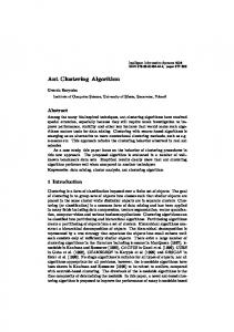
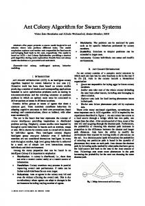
Figure 2. The process of clustering of A4C (a) Initial data distribution in the grid (b) Agents’ distribution after 0 iterations (c) Agents’ distribution after 10000 iterations (d) Agents’ distribution after 20000 iterations
(d)
Figure 1. The process of clustering of LF algorithm (a) Data distribution in the attribute space. (b) Initial data distribution in the grid (c) Data distribution after 500000 iterations (d) Data distribution after 1000000 iterations In Lumer and Faieta’s experiment a 100×100 grid was used and the initial distribution of the agents in the grid is as shown in Fig. 2(b). Fig. 2(c) and Fig. 2(d) show the data distribution after 500000 and 1000000 iterations respectively. The parameters used in the test are k1 = 0.1, k 2 = 0.15, α = 0.5, s 2 = 9 . We test the same benchmark using our algorithm A4C. Fig. 2(a) shows the clustered data while Fig. 2(b) shows the initial distribution of the agents in the grid. Fig. 2(c) and (d) show the agents’ distribution after 10000 and 20000 iterations respectively. In the test the parameters are set as: t max ← 2×10⁵ , sx ←1, s y ←1, θ ← 0.90, kα = 0.50, kλ = 1 . initial value of α in (6) is 0.5486, and k t λ(t) = 2 + λ lg max . In each iteration, the value of α is t ft updated adaptively by formula α(t) =α(t −50) −kα( ft − ft−50) . In The
the movement, the agent selects its destination using greedy method.
The figures show that the LF algorithm costs much more computation time than ours. The reason is that LF algorithm spends much time for the ants to search for the proper location to pickup or drop the data objects.
4.2. Real Data Sets Benchmark We test LF and A4C using the real benchmark of Iris. In the test, we consider two types of A4C: one sets the parameters adaptively and we still denote it as A4C, the other uses constant parameters and we call it SA4C (special A4C). Large amount experimental results that the A4C clustering results after 5000 iterations are mostly better than those of LF after 1000000 iterations. We set the parameter tmax the maximum iterations of LF algorithm as 1000000, and those for A4C and SA4C as 5000. We set the parameters k1=0.10, k2=0.15 in LF and set θ=0.9, λ=2,kα=0.5, kλ=1 in SA4C and A4C. We also set the initial 4 4 α value of A C as 0.4483 and the α value of A C as 0.30. In the three algorithms, we set the size of the neighbor as 3×3. Results of 100 trials of each algorithm on the Iris data set are shown in Tab. 1. It can easily be seen from Tab. 1 that SA4C and A4C require less iteration than LF. The quality of the clustering of SA4C is better than LF, but is worse than A4C.
1391
Proceedings of the Third International Conference on Machine Learning and Cybernetics, Shanghai, 26-29 August 2004 parameters are selected and adjusted adaptively. It has fewer restrictions on parameters, requires less computational cost, and has better clustering quality. Experimental results on standard clustering benchmarks demonstrate the ASM and A4C are more direct, easy to implement, and more efficient than BM and LF.
Table 1. Parameters and test results of LF, SA4C and A4C on Iris (100 trials) LF SA4C A4C Maximum iterations tmax
1000000
5000
5000
Minimum errors
3
3
1
References
Maximum errors
13
9
5
Average errors
6.68
4.41
1.97
Percentage of the errors
4.45%
2.94%
1.31%
Average running time(s)
56.81
1.34
1.42
[1] Bonabeau E., Dorigo M., Théraulaz G., Swarm Intelligence: From Natural to Artificial Systems. Santa Fe Institute in the Sciences of the Complexity, Oxford University Press, New York, Oxford, 1999. [2] Kennedy J., Eberhart R.C., Swarm Intelligence. San Francisco, CA: Morgan Kaufmann Publishers. 2001. [3] Dorigo M., Maniezzo V., Colorni A., Ant system: optimization by a colony of cooperative learning approach to the traveling agents[J]. IEEE Trans. On Systems, Man, and Cybernetics, 1996, 26(1):29-41 [4] Di Caro G., Dorigo M., AntNet: A mobile agents approach for adaptive routing, Technical Report, IRIDIA 97-12, 1997 [5] Von Neumann J., The general and logical theory of automata. In:AA Taub. Von Neumann J., Collected Works. Urbana: University of Illinois, 1963. 288~298. [6] Deneubourg, J.-L., Goss, S., Franks, N., Sendova-Franks A., Detrain, C., Chretien, L. “The Dynamic of Collective Sorting Robot-like Ants and Ant-like Robots”, SAB’90 - 1st Conf. On Simulation of Adaptive Behavior: From Animals to Animats, J.A. Meyer and S.W. Wilson (Eds.), 356-365. MIT Press, 1991. [7] Lumer E., Faieta B., Diversity and adaptation in populations of clustering ants, in: J.-A.Meyer, S.W. Wilson(Eds.), Proceedings of the Third International Conference on Simulation of Adaptive Behavior: From Animats, Vol.3, MIT Press/Bradford Books, Cambridge, MA, 1994, pp.501~508. [8] Handl, J. and Meyer, B., Improved ant-based clustering and sorting in a document retrieval interface, PPSN VII, LNCS 2439, 2002. [9] http://www.maslow.org/
In the LF algorithm, the agents make large amount of idle moving and the parameters are not adaptively selected, it takes quite a long time to converge. Moreover, the parameters in LF algorithm is hard to select especially the parameter α is very sensitive and can affect the quality of clustering result. In our algorithm, the agents move effectively, the parameters are selected and adjusted adaptively. It has fewer restrictions on parameters, requires less computational cost, and has better clustering quality. 5.
Conclusion
An artificial Ants Sleeping Model (ASM) is presented to resolve the clustering problem in data mining by simulating the behaviors of gregarious ant colonies. In the ASM mode, each data is represented by an agent. The agents’ environment is a two-dimensional grid where each agent interacts with its neighbors and exerts influence on others. Those with similar features form into groups, and those with different features repel each other. In addition, we proposed effective formulae for computing the fitness and activating probability of agents based on the ASM model. We also present an Adaptive Artificial Ants Clustering Algorithm (A4C). We also proposed several ants moving strategies for A4C that have salient effect in fastening the clustering process. In A4C, the agents can form into high-quality clusters by making simple moves according to little local neighborhood information and the
1392