An Adaptive Bayesian Approach to Dose ... - Statistical Science

An Adaptive Bayesian Approach to Continuous Dose-Response Modeling

Thomas J. Leininger

A selected project submitted to the faculty of Brigham Young University in partial fulfillment of the requirements for the degree of Master of Science

C. Shane Reese Gilbert W. Fellingham Scott D. Grimshaw

Department of Statistics Brigham Young University April 2010

Copyright © 2009 Thomas J. Leininger All Rights Reserved




ABSTRACT An Adaptive Bayesian Approach to Continuous Dose-Response Modeling

Thomas J. Leininger Department of Statistics Master of Science Clinical drug trials are costly and time-consuming. Bayesian methods alleviate the inefficiencies in the testing process while providing user-friendly probabilistic inference and predictions from the sampled posterior distributions, saving resources, time, and money. We propose a dynamic linear model to estimate the mean response at each dose level, borrowing strength across dose levels. Our model permits nonmonotonicity of the dose-response relationship, facilitating precise modeling of a wider array of dose-response relationships (including the possibility of toxicity). In addition, we incorporate an adaptive approach to the design of the clinical trial, which allows for interim decisions and assignment to doses based on dose-response uncertainty and dose efficacy. The interim decisions we consider are stopping early for success and stopping early for futility, allowing for patient and time savings in the drug development process. These methods complement current clinical trial design research.

Keywords: dynamic linear models, Markov chain Monte Carlo (MCMC), Gibbs sampling, Phase II clinical drug trials, adaptive trial design




ACKNOWLEDGEMENTS Anyone who reads the following pages must know that they would not exist were it not for teachers and parents. Dr. Shane Reese thankfully took a chance on me and involved me in research early in my education. He sparked my passion for learning and exploring statistics. Other teachers were similarly important in contributing to my education and further convincing me that statisticians are actually pretty cool people. My parents have done more for me than I know to thank them for. They taught me to always achieve my best and have always been supportive of my goals. I also thank my wife, Alyse, for her constant support and faith in me.




CONTENTS

CHAPTER 1 Introduction

1

2 Literature Review

4

2.1

Introduction . . . . . . . . . . . . . . . . . . . . . . . . . . . . . . . . . . . .

4

2.2

Binary versus Continuous Response . . . . . . . . . . . . . . . . . . . . . . .

4

2.3

Bayesian Methods . . . . . . . . . . . . . . . . . . . . . . . . . . . . . . . . .

5

2.3.1

Introduction to Bayesian Methods . . . . . . . . . . . . . . . . . . . .

5

2.3.2

Bayesian Methods in Clinical Trials . . . . . . . . . . . . . . . . . . .

6

2.4

Markov Chain Monte Carlo . . . . . . . . . . . . . . . . . . . . . . . . . . .

7

2.5

Dynamic Linear Models . . . . . . . . . . . . . . . . . . . . . . . . . . . . .

8

2.6

Adaptive Design

. . . . . . . . . . . . . . . . . . . . . . . . . . . . . . . . .

9

2.6.1

Adaptive Allocation . . . . . . . . . . . . . . . . . . . . . . . . . . .

10

2.6.2

Stopping Rules . . . . . . . . . . . . . . . . . . . . . . . . . . . . . .

11

Summary . . . . . . . . . . . . . . . . . . . . . . . . . . . . . . . . . . . . .

13

2.7

3 Methods

14

3.1

Introduction . . . . . . . . . . . . . . . . . . . . . . . . . . . . . . . . . . . .

14

3.2

Four-Parameter Logistic Model . . . . . . . . . . . . . . . . . . . . . . . . .

16

3.2.1

4PL Parameter Interpretations

. . . . . . . . . . . . . . . . . . . . .

16

3.2.2

4PL Priors . . . . . . . . . . . . . . . . . . . . . . . . . . . . . . . . .

17

3.2.3

Metropolis-Hastings Sampling for 4PL Parameters . . . . . . . . . . .

19

Dynamic Linear Model . . . . . . . . . . . . . . . . . . . . . . . . . . . . . .

20

3.3.1

Notation—DLM . . . . . . . . . . . . . . . . . . . . . . . . . . . . . .

20

3.3.2

Likelihood—DLM Model . . . . . . . . . . . . . . . . . . . . . . . . .

21

3.3

iv

3.4

3.5

3.3.3

Prior Distributions—DLM Model . . . . . . . . . . . . . . . . . . . .

21

3.3.4

Complete Conditionals—DLM . . . . . . . . . . . . . . . . . . . . . .

22

Adaptive Design

. . . . . . . . . . . . . . . . . . . . . . . . . . . . . . . . .

24

3.4.1

Adaptive Allocation . . . . . . . . . . . . . . . . . . . . . . . . . . .

24

3.4.2

Interim Analyses . . . . . . . . . . . . . . . . . . . . . . . . . . . . .

26

3.4.3

Implementation of Adaptive Design . . . . . . . . . . . . . . . . . . .

28

Proposed Experiment . . . . . . . . . . . . . . . . . . . . . . . . . . . . . . .

29

4 Results

30

4.1

Adaptive Design Example: Evolution of a Trial . . . . . . . . . . . . . . . .

30

4.2

Preliminary Work: Determining Stopping Thresholds U and L . . . . . . . .

31

4.3

Simulation Results . . . . . . . . . . . . . . . . . . . . . . . . . . . . . . . .

33

4.3.1

Null Response and Slowly Increasing Example Trials . . . . . . . . .

34

4.3.2

Simulation Study: Operating Characteristics . . . . . . . . . . . . . .

43

4.3.3

Simulation Study: Patient Assignment . . . . . . . . . . . . . . . . .

43

4.3.4

Null Response Curve (Control) . . . . . . . . . . . . . . . . . . . . .

46

4.3.5

Monotone Slowly Increasing Curve . . . . . . . . . . . . . . . . . . .

47

4.3.6

Monotone Quickly Increasing Curve . . . . . . . . . . . . . . . . . . .

49

4.3.7

Nonmonotone Curve . . . . . . . . . . . . . . . . . . . . . . . . . . .

50

5 Conclusions 5.1

52

Discussion of Proposed Approach . . . . . . . . . . . . . . . . . . . . . . . .

52

5.1.1

Efficacy of the Dynamic Linear Model . . . . . . . . . . . . . . . . .

52

5.1.2

Efficacy of the Adaptive Design Approach . . . . . . . . . . . . . . .

53

5.1.3

Cost Comparison . . . . . . . . . . . . . . . . . . . . . . . . . . . . .

54

5.2

Future Research Opportunities . . . . . . . . . . . . . . . . . . . . . . . . . .

55

5.3

Closing Summary . . . . . . . . . . . . . . . . . . . . . . . . . . . . . . . . .

56

v

APPENDIX A Computational Code in R

62

A.1 Adaptive DLM Approach . . . . . . . . . . . . . . . . . . . . . . . . . . . . .

62

A.2 Fixed DLM and 4PL Approach . . . . . . . . . . . . . . . . . . . . . . . . .

66

vi

TABLES

Table 3.1

Prior parameter values for 4PL model . . . . . . . . . . . . . . . . . . . . . .

3.2

Adaptive design interim stopping decisions considered after each batch of patients.

4.1

. . . . . . . . . . . . . . . . . . . . . . . . . . . . . . . . . . . . .

26

The effect of varying U on trial decision in the control case. We want to control the Type I error rate at α = 0.05, which is achieved when U =99.9%.

4.2

19

32

The effect of varying L on trial decision for effective dose-response curves. We chose L = 60% because it will minimize trial length without any significant Type II error. . . . . . . . . . . . . . . . . . . . . . . . . . . . . . . . . . . .

4.3

32

AdDLM’s stopping decisions from 1,000 trials for each response curve. The dynamic linear model has a 3.8% Type I error and a maximum Type II error rate of 4%.

4.4

. . . . . . . . . . . . . . . . . . . . . . . . . . . . . . . . . . . .

43

Average sample sizes per trial for each curve and modeling approach (AdDLM or fixed design). For the adaptive model, higher relative sample sizes per treatment reflect (as desired) the dosages where the drug is most effective. Average total sample sizes per trial show a large savings is achievable through adaptive design. Known ED95 doses are indicated by ∗ . . . . . . . . . . . . .

45

4.5

Null response curve Type I error rates for the different approaches. . . . . .

47

4.6

Null response curve σ 2 estimation. . . . . . . . . . . . . . . . . . . . . . . . .

47

4.7

Null response curve τ 2 estimation (there is no known value with which we can compare). . . . . . . . . . . . . . . . . . . . . . . . . . . . . . . . . . . . . .

48

4.8

Slowly increasing curve Type II error rates by approach. . . . . . . . . . . .

48

4.9

Slowly increasing curve σ 2 estimation. Our values are slightly inflated from Table 4.6. . . . . . . . . . . . . . . . . . . . . . . . . . . . . . . . . . . . . .

49

vii

4.10 Slowly increasing curve τ 2 estimation . . . . . . . . . . . . . . . . . . . . . .

49

4.11 Quickly increasing curve Type II error rates. Only the AdDLM F -test rate shows a large difference from Table 4.8.

. . . . . . . . . . . . . . . . . . . .

50

4.12 Quickly increasing curve σ 2 estimation . . . . . . . . . . . . . . . . . . . . .

50

4.13 Quickly increasing curve τ 2 estimation . . . . . . . . . . . . . . . . . . . . .

50

4.14 Nonmonotone curve Type II error rates. We see a substantial advantage in the Type II error t-test error rates for the DLMs over the more rigid 4PL model.

. . . . . . . . . . . . . . . . . . . . . . . . . . . . . . . . . . . . . .

51

4.15 Nonmonotone curve σ 2 estimation

. . . . . . . . . . . . . . . . . . . . . . .

51

4.16 Nonmonotone curve τ 2 estimation

. . . . . . . . . . . . . . . . . . . . . . .

52

5.1

Cost savings potential from adaptive design in place of a fixed design approach. Costs represent estimated costs of currently ongoing clinical trials in the United States. . . . . . . . . . . . . . . . . . . . . . . . . . . . . . . . . .

56

viii

FIGURES

Figure 1.1

Example dose-response curves under the traditional binary-response model and our proposed continuous-response model. . . . . . . . . . . . . . . . . .

3.1

2

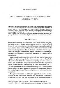
Possible dose-response scenarios for different drugs. The null response case is the control, while the slowly increasing, quickly increasing, and nonmonotone curves represent effective drugs with varying dose-response relationships. . .

3.2

Visual illustration of the traditional four-parameter logistic (4PL) model’s parameters. Note the monotonicity and smoothness inherent in the model. .

4.1

15

17

Flowchart for an adaptive design trial using the DLM (AdDLM approach). Patients are assigned in batches and stopping rules are assessed after each batch until one of the stopping requirements is met.

4.2

. . . . . . . . . . . . .

RA Stages 1–2 of an AdDLM trial for the null response curve. The drug is known to exhibit no effect at any dosage.

. . . . . . . . . . . . . . . . . . .

34

. . . . . . . . . . . . . . . . . .

35

4.3

RA Stages 3–6 for the null response curve.

4.4

RA Stages 7–10 of an AdDLM trial for the null response curve. The drug is known to exhibit no effect at any dosage.

4.5

. . . . . . . . . . . . . . . . . . .

36

RA Stages 11–14 of an AdDLM trial for the null response curve. The trial stops for futility after 14 RA stages, using a total of 226 patients. . . . . . .

4.6

31

37

Comparison of null response curve outcomes under the three modeling approaches. The 4PL model gives the tightest credible intervals, yet the DLMs allow more flexibility (the DLMs are less smooth).

4.7

4.8

. . . . . . . . . . . . . .

38

The first two allocation stages of an AdDLM trial for the slowly increasing response curve. . . . . . . . . . . . . . . . . . . . . . . . . . . . . . . . . . .

39

RA Stages 3–6 for the slowly increasing curve.

40

. . . . . . . . . . . . . . . .

ix

4.9

RA Stages 7–9 for the slowly increasing curve. The AdDLM model stopped for success after only nine batches of patients (using 176 total patients).

. .

41

4.10 Comparison of slowly increasing dose-response curve outcomes under the three approaches. The Fix4PL model again achieves smaller credible intervals, while the DLMs again have wider intervals and are more flexible. . . . . . . . . . .

42

x

1. INTRODUCTION

“The FDA is . . . responsible for advancing the public health by helping to speed innovations that make medicines and foods more effective, safer, and more affordable; and helping the public get the accurate, science-based information they need to use medicines and foods to improve their health.” (FDA mission statement) The U.S. Food and Drug Administration (FDA) is involved in a wide array of activities; this work will focus on its work in the development and regulation of new drugs. The FDA is charged with ensuring that drugs brought to the market are both safe and effective. Fulfilling this responsibility requires extensive testing to study possible side effects and to find the most effective dosage level. The several phases or trials of testing include substantial testing on humans. In the past, these trials have included mass testing at many dosage levels until the most effective dosage level is found, providing empirical observations about a population with little to say about the individual. The traditional dose-response curve is based on the probability of a treatment’s success, using a logistic model (see Figure 1.1). Such an approach is useful in many cases, but requires that the relationship follow the general parametric form of the model. Though logistic models do exist for continuous responses, they are not as common. This paper expands the traditional binary response curve into a continuous, possibly nonmonotone response curve, which will provide more flexibility given its semiparametric nature. This approach is more appropriate for situations where the measurement of interest is not a failure or success situation but a continuous spectrum of responses. Figure 1.1 below shows a comparison between a standard logistic dose-response curve for binary outcomes and the proposed semiparametric dose-response curve for continuous outcomes. As an example, the first model would be used to model the likelihood of a trial drug providing a successful amount of reduction in a patient’s blood pressure according to

1

the dosage received. The second model, however, would be used to measure the change in a

15 10 5

0.5

20

Proposed Continuous Model Reduction in Blood Pressure

Traditional Binary Model

0.0

Probability of a Successful BP Reduction

1.0

patient’s blood pressure after using the drug.

Log(Dose)

Dose

Figure 1.1: Example dose-response curves under the traditional binary-response model and our proposed continuous-response model.

The flexibility of the model also allows for nonmonotonicity in the dose-response curve, rather than forcing a monotonically increasing response, as is often assumed. Nonmonotonicity might occur, for example, if a drug’s benefit increases with the dose until a certain point, after which the drug becomes toxic. This proposed dose-response curve is fit by a Bayesian model, where an individual’s response to the drug at treatment level i is defined as yi and
yi ∼ N ormal θi , σ 2 . The parameters of the model, θ, σ 2 , and τ 2 , are estimated using Markov chain Monte Carlo (MCMC) methods, updating the posterior distributions of our parameters as patients are tested. The traditional trial design with equal sample sizes at each treatment is engineered to provide sufficient power to make statistical inference about the best dose. This method may not be the best or most efficient approach, however, as many patients may be receiving a marginally beneficial or even toxic treatment. The Bayesian framework of the proposed 2

model makes adaptive design, the current frontier in clinical trial design, an attractive alternative. Adaptive design is employed in this case by starting with a small, equal sample size for each treatment. The posterior distributions are then calculated for each parameter using MCMC, providing an intermediary assessment of the drug’s efficacy at each treatment level. A set of stopping rules is then assessed to decide whether the trial should continue or not. If the trial continues, another group of patients is then assigned to the treatments, with the probability of a patient being assigned to a treatment being proportional to the treatment’s efficacy. In this manner adaptive design provides a potentially more efficient approach that concentrates patients on more effective treatments and terminates the trial once conclusive evidence is received. Furthermore, the Bayesian framework cooperates seamlessly with the adaptive design of the trial. This will be discussed in more detail later. This thesis will discuss the opportunities provided by an adaptive Bayesian approach to dose-response modeling. The adaptive design allows for concentrating patients on more effective doses and for the possibility of stopping the trial early if enough information has been acquired. The Bayesian framework allows for improved personalization of the results and efficient implementation of the adaptive design. Any improvement in the efficiency of drug trials will save large amounts of time and resources, resulting in millions of dollars in savings and in more effective drugs on the market.

3

2. LITERATURE REVIEW

2.1

Introduction Clinical trials rely heavily on statistical design to provide a structure for sound decision-

making about the potency of experimental drugs. A typical Phase II clinical trial involves determining which dosages should be investigated and how patients react to the drug at those specified doses. This involves testing a range of doses in order to establish the efficacy of the drug across the range. There are many aspects of a Phase II trial design and therefore many considerations when setting up a trial. We now examine some aspects of clinical trials that we consider adapting in order to improve the efficiency and accuracy of Phase II trials.

2.2

Binary versus Continuous Response Responses in a typical dose-response study are modeled in a binary fashion. An out-

come is either labeled as a “success” or a “failure”; analyses are then performed to estimate the ability of each dose to provide a “successful” outcome. Though binary-response models are common, in many situations responses are originally measured in a continuous fashion. Crump (2002) proposes setting a threshold to divide continuous responses into two groups, providing a binary structure. Sand, von Rosen, and Filipsson (2003) investigate further how the choice of a threshold affects a study’s conclusions. Although there may be many benefits to having outcomes modeled in a binary manner, much research is now being done to assess how best to model continuous responses in their original, continuous form. Simon (1999) provides an early example in modeling continuous responses in active control clinical trials. Using the raw responses rather than a conversion into a binary structure, Simon compares the posterior probabilities of the treatment being superior to the control to determine a drug’s efficacy.

4

One goal of this work is to provide a reference for modeling continuous responses and to explore the benefits of modeling outcomes in their continuous state. This methodology will allow inferences about observing responses in any chosen interval or above some desired level of effect. Such inferences will provide doctors with more information when making diagnoses. Patients would also benefit from having a more personalized diagnosis and would therefore be expected to achieve better health.

2.3 2.3.1

Bayesian Methods Introduction to Bayesian Methods An essay by Reverend Thomas Bayes in 1763 proved to have a profound effect on

the outlook of statistics. His well-known rule, allowing him to find a solution to an inverse probability problem, became the basis for a new realm of statistics that would be developed over the centuries following his death. The basis for Bayesian inference is to combine a prior distribution for each parameter of interest with the likelihood function to get the posterior distribution for each parameter. Assuming a parameter has a distribution rather than being some unknown constant violates traditional frequentist views. Ashby gives three explanations for the use of prior distributions: “as frequency distributions based perhaps on previous data, as normative and objective representations of what it is rationale [sic] to believe about a parameter, or a subjective measure of what a particular individual actually believes” (2006, p. 2590). Using information from both the prior belief and the observed data, the posterior distribution gives an updated knowledge about each parameter’s distribution. We then utilize the posterior distributions to make inferences about each parameter, though the posterior distributions can often be examined only through numerical methods. Bayesian analyses were therefore very limited until recent developments in computers and computational methods. However, full-scale Bayesian trials are now possible, provided trial statisticians are knowl-

5

edgeable enough to implement Bayesian methods correctly. The recency of the development of Bayesian methods has made many skeptical of the accuracy and validity of Bayesian analysis, causing much debate (Berry 2005a; Howard, Coffey, and Cutter 2005; Moye 2008).

2.3.2

Bayesian Methods in Clinical Trials Ashby (2006) gives a 25-year review of the uses and innovations regarding Bayesian

statistics in medicine. Ashby notes that Cornfield has been a strong proponent of using a Bayesian paradigm in clinical trials since the 1960s (Cornfield, Halperin, and Greenhouse 1969; Ederer 1982). However, Bayesian advocates were “hampered by the lack of computational power, affecting both the nature of the problems tackled, and . . . the depth to which analysis could be pursued” (Ashby 2006, p. 3592). Bayesian outlooks played a supporting role to the more feasible existing methods. A great influx of books and articles regarding Bayesian methods and techniques for their implementation beginning in the 1990s made Bayesian statistics more viable for complex analyses. Particularly instrumental was the development of the Markov chain Monte Carlo (MCMC) algorithm for estimating posterior densities, as discussed later. Developments of Bayesian methods in many areas, such as medical technology, have made evident the potential of Bayesian methods, opening the way for Bayesian methods to take a more prominent role in clinical drug trials. Donald Berry, a strong proponent of using Bayesian designs in clinical trials, suggests that “the Bayesian paradigm is tailored to the learning process” (2005a, p. 1621). Inferences can be made at any time and with whatever information is available. He further suggests that the subjectivity in the choice of a model is essential; frequentists introduce subjectivity in the choice of the model, which may have a bigger impact than the choice of the prior in a Bayesian framework. Berry also adds that a flat or noninformative prior specification can be used to preserve the frequentist attitude, if desired, but still have the flexibility of the Bayesian structure.

6

Other opportunities provided by a Bayesian design are the abilities to learn sequentially, to borrow strength and information across studies and patient subgroups, and to provide predictive probabilities of future results (Berry 2005b). Berry, Carroll, and Ruppert (2002) investigate the effect of prior misspecifications in a simulation study and find that, at least in that case, the results prove robust to minor distributional misspecification. Howard (2005) expresses concern about the specification of prior distributions for clinical trials. What if there is disparity about what is really “known” previous to the trial? Will the study sponsor, who has a financial stake in the outcome of the trial, optimistically bias the treatment’s prior specification, thereby biasing the inference? He further suggests that Bayesian Phase III trials should not use Phase II data, arguing that each trial phase should be an independent confirmation of previous work. The abundance of debate surrounding application of the Bayesian paradigm in clinical trial design is indicative of the need to further study the advantanges and disadvantages of such a design. We will examine the efficiency and accuracy of a Bayesian clinical trial via a simulation study.

2.4

Markov Chain Monte Carlo The estimation of the parameters of the Bayesian response model will require Markov

chain Monte Carlo (MCMC) methods to sample from the joint posterior distribution of the parameters. By sampling from the complete conditional density of each parameter, we eventually converge to getting samples from the marginal posterior densities of each parameter, which combined comprise the joint posterior distribution. These samples from the joint posterior allow inference concerning the efficacy of the drug at each dosage level. Hastings (1970) introduces MCMC as a more efficient numerical computation method. He describes how to sample from the stationary distribution of a Markov chain and discusses assessing the error of MCMC estimates. Building on Hastings’ methods, Geman and Geman (1984) introduce Gibbs sampling as a way to get samples from the marginal densities using 7

conditional densities. They also prove that those iterative densities converge to the true densities, as long as each density is visited indefinitely often (no particular order is needed). Gelfand and Smith (1990) further discuss previous work on Gibbs sampling as well as provide concrete examples of implementations of the sampling algorithm. From these three works we get a framework where we can iteratively sample from the complete conditional distribution f (θi | x, θ−i ) of each θi , where θ−1 defines the collection of all parameters in θ except θi . The samples from f (θi | x, θ−i ) converge to samples from f (θi ), from which we can then make inference about the joint posterior distribution. Dodds and Vicini (2004) investigate the convergence of MCMC techniques in applied examples. They suggest a need for a unified decision on an integrated approach for determining convergence of MCMC chains. There are several existing methods, each stressing a certain aspect; therefore a combination of techniques ensures proper assessment of convergence properties.

2.5

Dynamic Linear Models One type of model in the dose-response realm worth an analysis is a dynamic linear

model (DLM). A dynamic linear model is essentially a simplified case of a Gaussian Process. The basis of a Gaussian Process is that each parameter is related in some way to the other parameters in the model. In a dose-response context this means that the true response to a treatment at one dosage level might be estimated using some weighted average of the estimates for the treatment’s effect at neighboring dosage levels. We could reasonably assume that a treatment’s effect could be monotone over small intervals, though it may be nonmonotone over the whole dosage space. Averaging the responses in a close proximity to the dose in question should thus give a sensible estimate for that dose’s true response. A similar structure is employed by Besag (1986) in reconstructing the true scene of an imperfect picture. Besag assumes that the color of any pixel could be estimated using 8

some function of the surrounding pixels and therefore maximizes his model according to the surrounding colors in an iterative fashion. Besag’s Iterative Conditional Modes model is shown to perform much better than the contemporary traditional maximum likelihood estimation process. Berry, Carroll, and Ruppert (2002) examine Gaussian Processes in the context of fitting a smoothing spline in a nonparametric regression setting. Their cubic estimator g of the true spline m is defined as the minimizer of a sum of squared errors; namely g minimizes Pn 2 i=1 {m(Xi ) − g(Xi )} . Their g estimator at each knot is a function of the estimator at all other knots. Liu and West (2009) use Bayesian dynamic linear models with Gaussian Process priors as a more flexible and computationally efficient approach to computer simulation in a hydrological system. They conclude that their approach is effective in estimating long time series trends that are dynamic in nature. They provide evidence that they are furthermore very useful in providing predictions of new design outcomes. Since the treatment response at one dosage level should be related in some way to responses to doses in a close proximity, we consider applying a dynamic linear model to estimate true dose-response relationships. The added strength gained from borrowing information from other dosage levels could potentially provide more information with fewer patients.

2.6

Adaptive Design There is no lack of motivation for improving the efficiency of clinical trials. Patients

and drug companies alike would benefit from any advances in trial design that would either provide better information about the drug’s nature or shorten the length of the trial. Scott Gottlieb (2006) of the FDA discusses the need for innovation in clinical trial design, especially in the area of adaptive design. This new approach to trial design allows clinical trials to preserve statistical rigor while also allowing a more dynamic structure of 9

the trial. Although relatively new, adaptive design has become the topic of much research and has begun to be implemented into actual clinical trials. The Acute Stroke Therapy by Inhibition of Neutrophils (ASTIN) study, by Krams et al. (2003), is the first major study that applies the principles of adaptive design in a full-scale Bayesian dose-response study. The study uses both adaptive allocation of patients and early stopping rules to improve the efficiency of the trial, studying fifteen dose levels in less time and with fewer patients than a traditional study of three dose levels.

2.6.1

Adaptive Allocation Patient allocation to treatments in a classical clinical trial involves choosing a sample

size that provides the desired power and then allocating the chosen number of patients to all treatments being studied. This provides a rigid structure in which the experiment is not altered during its course and all inference about the treatment is done after the testing is finished. This method, the current practice for most clinical trials, provides a constant error at every dose regardless of the outcome, but is arguably inefficient. Adaptive allocation of patients, available in both frequentist and Bayesian settings, is an alternative which makes use of intermediary information to steer the patient allocation in the trial. A much smaller group of patients is initially assigned to each dose. Interim evaluations then allow trial statisticians to assign patients to those doses that prove to be more effective, though in a manner that preserves the randomness of dose assignment. In a frequentist setting adaptive allocation requires the calculation of conditional power at each interim analysis to assess the new required sample sizes. Although a Bayesian analysis would not involve a power assessment, posterior probabilities (e.g., of being more effective than the control) are often used to assess the efficacy of different drug dosages and to steer patient allocation. Thall and Russell (1998), for example, implement an adaptive design feature in two Phase I/II dose-escalation examples. If the drug has not reached a significant efficacy, then

10

the dose is incremented, as long as it has not become toxic. Thall and Russell use the posterior probability of a drug reaching a certain level of effectiveness as a basis for determining whether a drug has reached a significantly effective level. Using an adaptive allocation approach, patients are more likely to receive effective doses than under the classic design. This benefit is a key point in Gottlieb’s 2006 address, which asks for adaptive methods that expose fewer patients to experimental treatments. Adaptive allocation presents an opportunity to improve patient treatment while simultaneously providing more information about the doses that prove to be most efficient. As adaptive allocation shows potential for great gains, this thesis will propose and evaluate a strategy for adaptively allocating patients.

2.6.2

Stopping Rules Perhaps the most significant aspect of adaptive design is the allowance for an experi-

ment to be ended once sufficient information about the drug’s potency has been collected. A drug might show significant efficacy at certain dosage levels, in which case continuing the trial would not sufficiently change the results already observed. The trial should arguably be stopped and started on the next phase. Alternatively, if a drug shows no effect at any dose at a point late in the trial, why should more patients be assigned to a futile trial? The argument that a trial should stop once a significant inference can be made is a main element of adaptive trial design. Early termination is an option in both frequentist and Bayesian designs, though the Bayesian paradigm incorporates the interim decisions more seamlessly. Bauer and Koenig (2006) examine using conditional power for interim decision-making in a frequentist setting. They suggest, however, that no general rules exist when making interim conditional power assessments, and therefore recommend that extra caution be taken. As mentioned previously, the ASTIN trial (Krams et al. 2003) is a pioneer in implementing both adaptive allocation and early termination rules in a Bayesian setting. The

11

ASTIN trial utilizes posterior probability bounds to determine whether a trial should end early, whether for success or futility. As the trial progressed, the drug failed to show any significant effect and the trial was therefore terminated for futility. This allowed the trial to study more doses while still reaching the same conclusion in less time. Thall and Simon (1994) further explain stopping rules in which they terminate the trial if the number of observed successful responses (in a binary response situation) exceeds predetermined critical limits, based on posterior probabilities. Thall and Simon suggest using a flat prior, highly concentrated around the control treatments prior, as a means to not allow an overly optimistic prior to lead to improper terminations for success when a drug has not sufficiently proven to be superior. Heitjan (1997) discusses similar stopping rules in the context of “Bayesian persuasion probabilities,” which he defines as the posterior probabilities of a therapy having a greater effect than the control. Heitjan formulates the early stopping rule as such: “In the case of acceptance, the data should convince a sceptic; in the case of rejection, the evidence should convince an enthusiast” (p. 1792). He therefore uses two prior specifications for each treatment—one which expects the new treatment to be better than the control and the other which assumes the treatment will be no better than the control. For the trial to be terminated for success, Heitjan’s pessimistic persuasion probability must exceed a certain upper limit. Similarly, the optimistic persuasion probability must drop below the lower limit for the trial to be terminated for futility. A health technology article by Spiegelhalter, Myles, Jones, and Abrams (1999) also suggests giving the treatments a skeptic prior, essentially a handicap the treatments must overcome in order to prove efficacy. Spiegelhalter et al. state that “the approach shows a degree of conservatism which can be remarkably similar to that of frequentist stopping rules” (p. 511). One final adaptive design option worth mentioning is applying a factorial design. Berry (2005b) suggests, given the long queue of drugs waiting to be tested, applying a combination

12

of drugs to groups of patients rather than making each drug wait in queue for its individual trial. In this manner drugs spend less time waiting to be tested and the odds of finding an effective drug increase dramatically. Given the high failure rate among drugs, clinicians can filter through ineffective drugs more quickly, speeding the testing process for effective drugs.

2.7

Summary As discussed in this chapter, many opportunities exist to investigate methods that

might lead to improved clinical trial design. A Bayesian framework provides a flexible model while allowing for continual updating of information as it is received as interim evaluations. MCMC methods will allow for efficient, reliable computation of the parameters of the Bayesian model. Adaptive allocation of the patients focuses patients on those doses that prove to be more effective. Finally, adaptive stopping rules allow a trial to terminate once enough information about a drug’s potency or lack thereof has been collected. The adaptive Bayesian framework presented in the next chapter, implementing the elements discussed in this chapter, supports current research needed in the clinical trial field.

13

3. METHODS

This chapter describes the general context of our experiment. A background to the context of our experiment is first given, followed by a description of how a traditional approach to clinical drug testing is performed. We then describe the components of our proposed approach, with regards to both dose-response modeling and trial design. Our Bayesian dynamic linear model (DLM) provides a method for improving the flexibility in dose-response modeling, while our proposed adaptive design allows for adaptive patient allocation to treatments and early stopping. Finally, an outline of the experiment comparing our approach to traditional methods is given. 3.1

Introduction Stacey and Reese (2007) explore a binary dose-response relationship that is modeled

as a parametric curve. In their approach, responses are dichotomized as either effective or not effective, with the parametric curve being strictly monotone. Our model expands their work, allowing the response to be continuous, and increases the flexibility of the dose-response relationship, allowing for nonmonotonicity. The context for testing our model will be within the framework of a clinical trial for a drug meant to reduce micturition frequency among patients. The response metric used for each individual is the difference in micturition frequency before and after using the drug, where a positive number reflects a reduction in micturition frequency, indicative of a beneficial effect for the patient. Our purpose is to assess our model’s validity and effectiveness in fitting the model by comparison to a known, prespecified dose-response relationship from which our data was generated. As our basis for comparison, we take curves presented in Berry (2002) as our known, prespecified dose-response curves. The various curves allow us to test our model under many scenarios. Included among the dose-response curves are a null response dose-

14

response curve, a slowly increasing monotone curve, a quickly increasing monotone flat curve, and most importantly, a nonmonotone curve. Figure 3.1 illustrates the dose-response relationships that are commonly encountered in this type of clinical trial. A drug might, for example, exhibit an increasing effect as the dose increases, shown by the slowly increasing curve (black curve). A second dose-response relationship might have a sharply increasing effect as increasing doses are applied, but then hold constant at a certain maximum effect once the dosage has been incremented above a certain threshold, illustrated by the quickly increasing curve (blue curve). Alternatively, a

3.5

●

●

●

●

●

●

●

3.0

● ● ●

2.5

Null Response Slowly Increasing Quickly Increasing Nonmonotone

● ●

2.0

●

● ●

●

1.5

●

●

●

● ●

●

0

10

●

●

●

40

80

●

●

●

120

160

200

1.0

Response (Change in Micturition Frequency)

drug might show no effect at any dose, represented by the null response curve (red curve).

Dose (in mg)

Figure 3.1: Possible dose-response scenarios for different drugs. The null response case is the control, while the slowly increasing, quickly increasing, and nonmonotone curves represent effective drugs with varying dose-response relationships.

The nonmonotone curve (green curve) presents yet another possible relationship in which increases in the dosage level lead to an increase in the drug’s effect up to a certain point, after which increases in the dosage lead to a decrease in the drug’s effect. This nonmonotone curve may reflect a drug that becomes toxic above certain dosages, and therefore not only has a decreased effect than at lower doses, but could potentially become harmful to the patient. 15

This work examines the capability of our methods to accurately and efficiently model any of these dose-response relationships. In the next chapter we will specifically examine our model’s performance on the four curves in Figure 3.1. Our special interest is assessing the flexibility of our model in estimating the wide variety of shapes of dose-response relationships found in Figure 3.1.

3.2

Four-Parameter Logistic Model In order to compare the estimation abilities of our proposed design dynamic linear

model to current models, we use a four-parameter logistic (4PL) model as a baseline. This logistic model is an extension of the typical binary response logistic model with which we can model continuous data. The general form of the model is Yi ∼ N ormal (E(Yi ), σ 2 ), where E(Yi ) = D +

A−D 1 + (Xi /C )B

(3.1)

and Xi is the dosage for treatment i. 3.2.1

4PL Parameter Interpretations The parameters A, B, C, and D do have simple interpretations, namely: • A is the minimum value of the mean response curve over the dosage range (assuming B is nonnegative), • B is the slope parameter, • C is the dosage for which the mean response curve achieves its mean value, and • D is the maximum value of the mean response curve as the curve goes toward infinity (assuming B is nonnegative).

16

100

150

200

4 3 2 1 0 0

50

100

Changing D A = 1, B = 1, C = 100

150

200

200

150

200

1

2

3

D=4 D = 2.5 D=1 D=0

0

3 2

100 Dose (in mg)

150

4

Changing C A = 1, B = 1, D = 4

1

50

B=1 B = 0.5 B=0 B = -0.5

Dose (in mg)

C = 100 C = 50

0

Changing B A = 1, C = 100, D = 4

Dose (in mg)

Response (Change in Micturition)

50

4

0

Response (Change in Micturition)

4 3 2 0

1

A=1 A=2

0

Response (Change in Micturition) Response (Change in Micturition)

Changing A B = 1, C = 100, D = 4

0

50

100 Dose (in mg)

Figure 3.2: Visual illustration of the traditional four-parameter logistic (4PL) model’s parameters. Note the monotonicity and smoothness inherent in the model.

A visual illustration of the parameters is given in Figure 3.2. We notice from Figure 3.2 that the four-parameter logistic curve does allow a wide variety of shapes, including even flat or decreasing relationships. In fact, each curve has two parameterizations: switching the values of A and D and making B negative produces an identical curve to one with the original values of A, B, and D. The four-parameter logistic model does not, however, allow any nonmonotonicity in the relationship, which we suggest can be fixed with our less rigid semiparametric DLM approach to modeling.

3.2.2

4PL Priors We expect the responses at each dosage to be distributed normally. As mentioned

previously, we are more interested in modeling the amount of reduction in micturition frequency (a continuous response) rather than whether there is a reduction (a binary response; see Stacey and Reese 2007).

17

As noted above, we assume that an individual’s response to the drug at each dose follows a Normal distribution, or yij ∼ N ormal (E(Yi ), σ 2 ). This implies an assumption of constant error for individual responses for all the doses, i = 0, 1, . . . , t. The likelihood function is ( f (y | A, B , C , D, σ 2 ) = (2πσ 2 ) where E(Yi ) = D +

−N 2

exp

−

Pt

i=0

Pni

2 j=1 (yij − E(Yi )) 2σ 2

) ,

A−D 1 + (Xi /C )B

and Xi is the dosage for treatment i. We choose prior distributions for A, B, C, D, and σ 2 which have support in agreement with the support of the parameters. C and σ 2 must have positive values, so their priors will not use Normal distributions, whereas A and D can reasonably be assumed to follow Normal distributions. We let C be greater than the maximum dose studied because doing so allows for a linear dose-response relationship across all the doses. The parameters are essentially indistinguishable (as noted above) unless we restrict B to be positive; therefore, B will not use the Normal distribution either. The prior distributions for all of our parameters are σ 2 ∼ Inverse Gamma (aσ , bσ ) , where E(σ 2 ) =

1 bσ (aσ − 1)

,

(3.2)

A ∼ N ormal (ma , s2a ), B ∼ Gamma (ab , bb ), where E(B) = ab bb , C ∼ T runcated N ormal (mc , s2c ), where 0 ≤ C < ∞, and D ∼ N ormal (md , s2d ). For our application, we chose the values shown in Table 3.1 for our prior parameters, based on our prior beliefs.

18

Table 3.1: Prior parameter values for 4PL model aσ bσ ma s2a ab

3.2.3

83 0.001355 0 1 1.00

bb mc s2c md s2d

1.00 100 50 0 1

Metropolis-Hastings Sampling for 4PL Parameters Using the prior distributions and likelihood function listed above, the joint posterior

is

   2  Pt Pni   A−D     − i=0 j=1 yij − D +   B −N 1 + (X /C ) i 2 2 2 f (σ , A, B , C , D | y) ∝(2πσ ) exp   2σ 2           −1 −(A − ma )2 2 −(aσ +1) × (σ ) exp × exp bσ σ 2 2(s2a )   −(C − mc )2 ab −1 ×B exp{−B/bb } × exp 2s2c   −(D − md )2 . (3.3) × exp 2s2d The complexity of the joint posterior in terms of A, B, C, and D makes solving for

closed form complete conditionals impossible, though it is possible to solve for the closed form complete conditional distribution of σ 2 . Therefore, we can only use Gibbs sampling on the complete conditional of σ 2 and we must use the Metropolis-Hastings (M-H) sampling algorithm on the rest of the parameters. Explanation of the M-H algorithm can be found in Hastings (1970). The complete conditional for σ 2 is  [σ 2 ] ∼ Inverse Gamma 

N + aσ , 2

ni  t 1 XX

1 + bσ 2

i=0 j=0

 yij − D +

A−D 1 + (Xi /C )B

2 !−1

 .

Once we get draws from the posterior distributions, we get a distribution for the mean response at each dosage Xi using Equation 3.1 and the invariance property of posterior 19

distributions. We will then use the posterior distributions of each dosage by comparing them to the same distributions as calculated using the dynamic linear model.

3.3

Dynamic Linear Model Our dynamic linear model (DLM) makes use of the Bayesian paradigm through an

MCMC simulation of the model’s parameters, such as the mean response at each dosage. We propose this model as a way to increase the flexibility in modeling dose-response relationships. Before presenting the model, however, we first present some notation.

3.3.1

Notation—DLM The following notation will be used throughout the paper: • yij = response of the j th individual at the ith dosage level, • y i = the mean observed response among all patients at the ith dosage level, • ni = number of patients who received the ith treatment, • t = total number of treatments, • N = total number of patients tested, • νi = dosage for the ith treatment (in mg), • di =

√ νi − νi−1 = square root of the distance between the current and previous

dosage levels, • θi = the mean response for the ith treatment; a positive response signifies a reduction in micturition; θ0 designates the mean response of the placebo or control treatment, • σ 2 = the variance of individuals about the mean response at each dosage level, and • τ 2 = the a priori variance of the mean response at each dosage level. 20

3.3.2

Likelihood—DLM Model The likelihood function is unchanged from the previous section, except that in the

dynamic linear model, E(Yi ) = θi , or yij ∼ N ormal (θi , σ 2 ). The likelihood function is now written as

( f (y|θi , σ 2 ) = (2πσ 2 )

3.3.3

−N 2

exp

−

Pt

i=0

Pni

2 j=1 (yij − θi ) 2σ 2

) .

Prior Distributions—DLM Model We fit a dynamic linear model that assumes that the mean response at each dose level

follows a normal distribution, but allows each dose’s distribution to have its own mean. Each dose has a hierarchical structure, with a common variance and a mean related to adjacent doses’ means. Dose level posterior distributions are updated as the data are incorporated into the modeling. Note that this allows for nonmonotonicity in the dose-response curves (such as the nonmonotone curve in Figure 3.1) and provides added flexibility to the model. Our dynamic linear model allows for increased flexibility and borrowing of strength across dosage levels, which will be more clear in the form of the complete conditionals. The dynamic linear nature comes from the fact that the distribution of θi is a function of θi−1 . Note that the prior distribution of θ0 must be specified with some initial parameter values, since θ−1 does not exist. Note also that the inclusion of the di term allows the model to appropriately adjust the strength borrowed from responses at neighboring doses as a function inversely related to their distance from the ith dose. A more concise statement of the model is θ0 ∼ N ormal (0, b) ,

(3.4)


θi ∼ N ormal θi−1 , di τ 2 , σ 2 ∼ Inverse Gamma (aσ , bσ ) , where E(σ 2 ) =

1

, and bσ (aσ − 1) 1 τ 2 ∼ Inverse Gamma (aτ , bτ ) , where E(τ 2 ) = . bτ (aτ − 1)

21

These distributions are chosen so that the support of the prior distribution matches that of the original parameter’s support. The priors also represent flexible distributions that allow a simplified computational algorithm, discussed in Section 3.3.4. Our model uses specific prior values of b = 2, aσ = 83, bσ = 0.001355, aτ = 3, and bτ = 0.5. Our specification of priors also centers the response at each dose around the mean for the previous dose’s mean; in other words, no automatic assumption of a higher dose having a higher efficacy is made.

3.3.4

Complete Conditionals—DLM A first step in developing a computational approach to estimate the dose-response

model in (3.4) is to solve for the complete conditional distribution of each unknown parameter. Solving for a closed form of the complete conditional distributions allows us to employ Gibbs sampling to acquire draws from the joint posterior distribution of our parameters. The joint posterior distribution then provides a basis for statistical inference and comparison between responses at each dose. The complete conditional distributions are  [θ0 ] ∼ N ormal  [θi ] ∼ N ormal

σ 2 d1 τ 2 b2 n0 d1 τ 2 b2 y 0 + σ 2 b2 θ1 , n 0 d 1 τ 2 b2 + σ 2 b2 + σ 2 d 1 τ 2 n 0 d 1 τ 2 b2 + σ 2 b2 + σ 2 d 1 τ 2

 ,

ni di di+1 τ 2 y i + σ 2 di+1 θi−1 + di σ 2 θi+1 di di+1 τ 2 σ 2 , ni di di+1 τ 2 + σ 2 di+1 + σ 2 di ni di di+1 τ 2 + σ 2 di+1 + σ 2 di

(3.5)

 ,

for i = 1, 2, ..., t − 1,  [θt ] ∼ N ormal

nt dt τ 2 y t + σ 2 θn−1 dt τ 2 σ 2 , nt dt τ 2 + σ 2 nt dt τ 2 + σ 2 

[σ 2 ] ∼ Inverse Gamma 

"

ni t 1XX

N + aσ , 2 2

i=0 j=1

 ,

(yij − θi )2 +

1 bσ

#−1   , and

22



"

t 1X 1 1 t 2  + aτ , (θi − θi−1 )2 + [τ ] ∼ Inverse Gamma 2 2 i=1 di bτ

#−1  .

We notice that the posterior distribution for each θi is a function of the mean of the data for the ith treatment, θi−1 , and θi+1 . This illustrates the ability of the model to borrow strength and to smooth the curve across all doses while still allowing nonmonotonicity. We also note that θ0 and θt have a slightly different complete conditional distribution since no θ0−1 or θt+1 doses exist. Therefore, both θ0 and θt will be expected to have a larger variance since strength can only be borrowed from one neighboring dose. Finally, we note that the mean of the distribution for each θ can now clearly be seen as a weighted average between the data and neighboring mean response parameters. As Geman and Geman (1984) state, the order of our sampling from the complete conditionals does not matter, as long as each one is visited indefinitely often. We will, however, visit each one in the order shown above. Specifically, we will take 110,000 samples from each complete conditional; the first 10,000 draws will be considered as “burn-in” and will therefore be discarded. The remaining 100,000 draws from each distribution constitute draws from the joint posterior distribution. Inference can now be made concerning the mean response at each dose level, the variability of individual responses at each dose, or the posterior probability of one dose observing a higher response than the control. We will also provide credible intervals describing probabilities of the mean response of each dose and prediction intervals describing the probabilities of an individual response for each dose. As mentioned previously, we can use the 4PL model to estimate each θi using (3.1). In this manner we compare the estimates for each θi between the two modeling approaches and determine the relative abilities of each approach.

23

3.4

Adaptive Design We now discuss modifications to the design of the experiment, made possible by our

Bayesian framework, that will allow for improved efficiency. The two modifications we consider are adaptive allocation of patients to doses and the potential for stopping a trial early, due to either determination of success or determination of trial futility.

3.4.1

Adaptive Allocation As discussed previously, adaptive allocation is a technique that makes use of the in-

termediary information as a trial progresses. Patients are sequentially assigned to the doses that prove to be more effective. The assignment preserves the randomness and blindness of dose assignment. An adaptive design trial starts with a small number of patients at each treatment and a placebo. The preliminary dose-response curve is then fit after observing the initial group of patients’ responses. Next, the doses are evaluated and a new batch of patients are assigned randomly to doses, with a higher probability to more efficacious doses (efficacious doses are defined below). Once the responses from the second batch of patients are received, the dose-response curve is recalculated using all the available information. Again the doses are evaluated and another batch of patients are assigned to the treatments, with greater probability to efficacious doses. The trial continues in this fashion, continually examining responses and assigning new batches of patients. Doses with the highest posterior mean responses are candidates for efficacious doses. However, a dose with a large variance in its posterior mean response distribution is also important from a statistical perspective. In this case, we have higher uncertainty about the mean response and therefore want more information at that dose. Thus a combination of the variance of the mean response and the relative efficacy of the dose is our metric in assigning a probability of assigning subjects to each dose.

24

Logistically, we make assignments according to the above scheme by creating a vector p, where pi contains the probability that a patient will be assigned to treatment i in the next batch. A certain portion of the new patients will automatically be assigned to the placebo so we keep improving our knowledge of the control. In particular, the probability of a nonplacebo dose receiving more patients is

pi =

P (θi > ED95)σθi , for i = 1, 2, . . . , t. t X [P (θi > ED95)σθi ]

(3.6)

i=1

We first calculate the posterior probability that the mean response at a dose level is greater than the mean response of the placebo. That probability is multiplied by σθi , the standard deviation of the mean response at each dose (n.b., σθi is different from σ 2 , t X the variance of individual responses). This value is then standardized so that pi = 1, i=1

meaning that each of the pi can now be used as a probability of assigning the next patient to dose i. We can now sample from p to get the random dose assignments for the next batch of patients. After the responses from each batch of patients are observed and the posterior probabilities are calculated, we update p to reflect the current information. Another batch of patients is assigned, and so the process continues.

3.4.2

Interim Analyses An additional component we add to our approach is the possibility of stopping once

we have reached a prespecified information threshold. For example, the data might strongly suggest that a dose is effective, even though only half of the patients have been used. At that point we will consider stopping the trial if we have enough evidence that the dose in question is significantly effective. Another consideration for stopping early is in a case where none of the doses seem to have a positive effect on the patients. If we can accurately predict earlier in the trial that the 25

treatments show no effect, we can stop the trial. This would significantly reduce the cost of clinical trials and, more importantly, spare patients from receiving an ineffective treatment. We start the trial by randomly assigning a batch of patients equally to each of the treatment levels and the placebo (control) dose. We denote the starting sample size of each dose with ns , which we set equal to twelve for this application. After observing the responses from this first group of patients, we use MCMC to estimate the dose-response curve. Before the next random assignment, we test the three stopping rules, described in detail below and summarized in Table 3.2. Table 3.2: Adaptive design interim stopping decisions considered after each batch of patients. Decision Condition Stop for success Stop if P (θED95 ≥ θ0 ) > U for any θi Stop for futility Stop if P (θi ≥ θ0 ) < L for all θi Stop for cap N ≥S Continue None of the above rules are met

First, we consider stopping the trial for success, meaning that at least one successful dose has been found. At this point, the trial would enter rigorous testing of the successful dose in a Phase III trial. A dose is labeled successful if the posterior probability that the mean response of the most likely ED95 dose is greater than the control exceeds a predefined limit U . This requires that we first calculate the most likely ED95 dose, θ95 , which is the dosage level which has the highest posterior probability of having a mean response above the ED95 level. The ED95 level is defined as ED95 = θ0 + 0.95(max{θi } − θ0 ). We define θED95 as θED95 = θj , such that P (θj > ED95) = max{P (θi > ED95)} for i = 1, 2, ..., t. We stop a trial when P (θED95 > θ0 ) > U , and we call this stopping for success. 26

Second, we stop the trial for futility if none of the doses show any improved efficacy over the placebo. The trial would end and no further testing would be performed. Many clinical trials fail after years of testing (e.g., the 2003 ASTIN trial); this implementation would allow a clearly futile trial to stop early, saving significant time and money. The trial is stopped for futility when the posterior probability of the most likely ED95 treatment’s mean response being more effective than the control is less than or equal to a specified limit L for all treatments. We call this stopping for futility. Finally, we stop the trial if the maximum number of allotted patients S has been used. Although this rule is clear in an actual clinical trial, the rule proves necessary in a simulation setting. In our study, S = 600. At this point, no doses have shown to be significantly more effective than a placebo. However, the drug has not proven to be totally ineffective. Specific decisions at this point must be made by the trial statisticians. We call this stopping for cap. If none of the above conditions are met, then the trial is continued. The next batch of patients is assigned to treatments in the manner described in the adaptive allocation section and the pattern continues. We denote the number of patients assigned to the placebo in each batch with np and the number of patients assigned to a treatment in each batch with nd . We assume a constant accrual of np + nd patients, though this might be adapted to be made variable throughout the trial. For this application, we set np = 3 and nd = 7, meaning that we assume a constant accrual rate of ten patients. The notion of adding trial patients in batches mirrors the typical accrual pattern of patients to a clinical drug trial. In a clinical trial, fixed or adaptive design, patients are tested sequentially. Initially, only a handful of patients might be tested each month. As the trial progresses, however, more patients are tested each month. In a fixed design clinical trial, however, the results are not analyzed until the full amount of patients are tested (unless the trial must be stopped to preserve the safety of the patients). An adaptive design not only matches the accrual of patients, but an early stopping decision will save the trial sponsor’s

27

money and time. Successful drugs can then move on to the next phase months before they normally would.

3.4.3

Implementation of Adaptive Design With the above framework now in place, we specify the exact procedures of the adaptive

portion of the trial. The first batch of patients will consist of 96 patients, 12 patients receiving the placebo and 12 at each of the seven treatment levels. Once their responses have been observed, the posterior distributions will be calculated using MCMC computation as described in Section 3.3.4. We then analyze the stopping rules, although we do not expect a trial to have met the stopping conditions at this point. If none of the stopping rules are met, the trial continues with the assignment of a new batch of ten patients to the treatments. Three of the patients will automatically be assigned to the placebo, while the remaining seven will be assigned to one of the seven treatments, allocated randomly by assigning the seven subjects to treatment i with probability pi as defined in (3.6). Once the responses from the newest batch of patients are measured, the dose-response curve will again be estimated and the stopping rules assessed. The trial will continue in this manner until one of the stopping rules is met. In pseudocode, the above explanation can be written as the following algorithm: Start of Trial (1) Assign ns patients to the placebo and each treatment. (2) Observe responses and perform MCMC to get posterior distributions for σ 2 , τ 2 , and each θi . (3) Evaluate stopping decisions. If one of the stopping criteria is met, proceed to Step 4. If none of the stopping rules are met, then: (a) Calculate the p vector using (3.6).

28

(b) Randomly allocate np patients to the placebo and nd patients to the treatments, using pi as the probability that treatment i gets the next patient. (c) Repeat Steps 2 and 3 again. (4) End of Trial. Make inference based on the stopping decision.

3.5

Proposed Experiment Although our approach (DLM with adaptive treatment allocation) has been con-

structed in a way that attempts to increase the flexibility and accuracy of the estimation of the dose-response relationship and simultaneously shorten the trial length, we seek assessment through a simulation study. We are interested in the performance of our approach under all four dose-response curves in Figure 3.1 as compared to typical approaches. For each curve, we compare the performance of three models: a classic four-parameter logistic model with fixed patient allocation, our dynamic linear model with fixed patient allocation, and our dynamic linear model with adaptive patient allocation. We are then able to separate the effects of our model versus the classic four-parameter logistic model and the fixed allocation versus adaptive allocation for each of the four curves. Our measures for comparison are the number of patients at each dose and the standard deviation of our estimated response at each dose.

29

4. RESULTS

Before the results from our simulation can be presented, we first walk through the evolution of an adaptive design trial. We then discuss our method for determining U and L, the upper and lower stopping thresholds for our stopping decisions. Next, we present two trial simulations, one for a drug demonstrating no effect in the patients (red curve in Figure 3.1) and one for a drug exhibiting a slowly increasing dose-response relationship (black curve in Figure 3.1), to illustrate how each trial is performed in our simulation study. We then present and explain the simulation results, comparing the performance of each approach under each dose-response relationship. 4.1

Adaptive Design Example: Evolution of a Trial We now give a look into the actual development of a clinical drug trial under the

adaptive design DLM approach. We will look at two of the proposed cases: the null response case and the slowly increasing response case. Figure 4.1 summarizes the flow of an adaptive design trial. As described in the previous chapter, this process is fairly simple. At the start of the trial, 12 patients are assigned to each of the treatments and the placebo. The dynamic linear model is fit and then the stopping rules are assessed. If none of the stopping criteria are met, then the trial goes to Random Assignment (RA) Stage 2 and more patients are assigned to the trial. Three patients are given the placebo. Seven patients are randomly assigned (with replacement) a treatment, with the seemingly more effective doses having a higher probability of receiving more patients. The dynamic linear model is fit again and the stopping rules are again evaluated. If they are still not met, then the trial loops back into the next RA stage. This process continues until one of the stopping rules is met and the trial ends. At this point, a decision

30

Trial starts Random Allocation (RA) Stage 1 ns patients to placebo and each treatment

Dynamic Linear Model Fitting (DLMF) Stage

Stopping Rule Assessment (SRA) Stage

No stopping rules met

Stopping rule met

RA Stage 2, 3, ...

np patients to placebo and nd patients to a treatment, assigning to treatment i with probability P (θi > ED95)σθi pi = !t [P (θi > ED95)σθi ] i=1 for i = 1, 2, . . . , t

Decision Stage – Trial ends

Figure 4.1: Flowchart for an adaptive design trial using the DLM (AdDLM approach). Patients are assigned in batches and stopping rules are assessed after each batch until one of the stopping requirements is met.

of futility is made. If the trial uses its allotted number of patients and no early stopping decision has been made, then the trial is labeled futile.

4.2

Preliminary Work: Determining Stopping Thresholds U and L We first concern ourselves with determining appropriate values for our early termi-

nation thresholds U and L. Recall that if P r(θED95 > θ0 ) > U , then we declare the trial successful and stop the trial early. If P r(θi > θ0 ) < L for i = 1, 2, . . . , t, then we declare the treatment ineffective and stop the trial early. To determine an appropriate U we assume a case where the drug has no effect, meaning that the dose-response curve is perfectly flat and that none of the treatments are effective. Typically, we choose U so that the probability of declaring the treatment effective is no more

31

than 5% in this control case, resulting in a 5% Type I error rate. Table 4.1 summarizes the decisions made in 200 trial simulations with varying values of U and with L equal to 60% (we will check appropriate values for L next). Table 4.1: The effect of varying U on trial decision in the control case. We want to control the Type I error rate at α = 0.05, which is achieved when U =99.9%. U 95.0% 99.0% 99.5% 99.9% 99.95%

Stopped for Success (Futility or Cap) 0.420 (0.580) 0.145 (0.855) 0.120 (0.880) 0.055 (0.945) 0.045 (0.955)

Our original supposition was that U should be close to 90% or 95%, yet our simulation showed that U should actually be closer to 99.9%. We therefore chose to use U = 99.9% in the rest of our work. To determine an appropriate value of L, we again use simulation to demonstrate a desirable Type II error rate. This means that we assume that there is a dose or range of doses that is effective and set L so that we limit how often the treatment is declared ineffective by our algorithm. To do this, we use the slowly increasing and nonmonotone curves and simulate trials with different values of L. We then examine the different outcomes to determine a proper value for L. The results are given in Table 4.2. Note that in these simulations, we set U = 99.9% as determined above. Table 4.2: The effect of varying L on trial decision for effective dose-response curves. We chose L = 60% because it will minimize trial length without any significant Type II error. L 40% 50% 60% 70%

Slowly Increasing Curve Nonmonotone Curve Stopped for Success / Futility / Cap Stopped for Success / Futility / Cap 1.00 / 0.00 / 0.00 1.00 / 0.00 / 0.00 1.00 / 0.00 / 0.00 1.00 / 0.00 / 0.00 1.00 / 0.00 / 0.00 1.00 / 0.00 / 0.00 0.995 / 0.005 / 0.00 0.98 / 0.02 / 0.00

32

Based on the results in Table 4.2, L = 60% achieves the Type II error rate we desire: using L = 60% lets us stop more unsuccessful trials early (a cap decision is worse than a futility) without changing the Type II error rate. Setting L = 50% also achieves an appropriate Type II error rate, but setting L = 60% will cut down on trial length without substantially affecting the Type II error rate. We already know that the chosen combination of U and L simultaneously achieves the desired Type I and Type II error rates from our simulations to choose U. Therefore U = 99.5% and L = 60% will be used throughout the remainder of this paper.

4.3

Simulation Results We now present the results from simulating 1,000 clinical drug trials in the twelve

different scenarios: • Null Response Curve (control; red curve in Figure 3.1) – Dynamic Linear Model with adaptive treatment design (AdDLM) – Dynamic Linear Model with fixed treatment design (FixDLM) – Four-Parameter Logisitic Model with fixed treatment design (Fix4PL) • Slowly Increasing Curve (black curve in Figure 3.1) – AdDLM – FixDLM – Fix4PL • Quickly Increasing Curve (blue curve in Figure 3.1) – AdDLM – FixDLM – Fix4PL • Nonmonotone Curve (green curve in Figure 3.1) – AdDLM – FixDLM – Fix4PL

33

A summary of the effectiveness of the adaptive design and DLM approaches will be given afterwards. AdDLM will refer to the adaptive design dynamic linear model approach. FixDLM refers to the fixed design dynamic linear model approach. Fix4PL refers to the fixed design four-parameter logistic approach. We first give an example of how one trial evolves in both the null response and the slowly increasing cases, so the reader can better understand the adaptive design approach’s differences from the fixed design approach. We then give summaries of the two most important, overarching analyses of the relative performance of the three models and how our proposed approach compares. We finally look at each dose-response curve and compare the different approaches with more specialized metrics.

4.3.1

Null Response and Slowly Increasing Example Trials We first introduce an example where we test a drug that has no effect at any dosage

level. A placebo effect might be present, but it will be exhibited at each dose, and no added benefit from the drug at any dosage will be present. Figure 4.2 shows intermediary results of the trial after each dynamic linear model fitting (DLMF) stage.

Response (change in mict.)

RA Stage 2

Response (change in mict.)

RA Stage 1

0

20

40

80

120

Dosage (in mg)

160

200

0

20

40

80

120

160

200

Dosage (in mg)

Figure 4.2: RA Stages 1–2 of an AdDLM trial for the null response curve. The drug is known to exhibit no effect at any dosage.

34

The dose-response curves in Figure 4.2 show the estimated mean response of the patients at each dosage level, as well as a 95% credible interval for the mean response. The red dots along the x-axis each represent where the patient-assigning algorithm has randomly assigned patients to treatments. For example, in RA Stage 1, we see two red dots above the 200 mg dose, meaning that two patients will recieve the 200 mg dose treatment in the next round. The light gray dots each represent one patient’s response to the drug at the specified dosage (the plots do not show all of the responses, however, since many of the responses were more extreme than the desired plotting window). After the first two stages, we do not see any dosages that seem to show efficacy.

Response (change in mict.)

RA Stage 4

Response (change in mict.)

RA Stage 3

40

80

120

160

200

0

20

40

80

120

Dosage (in mg)

Dosage (in mg)

RA Stage 5

RA Stage 6

160

200

160

200

Response (change in mict.)

20

Response (change in mict.)

0

0

20

40

80

120

Dosage (in mg)

160

200

0

20

40

80

120

Dosage (in mg)

Figure 4.3: RA Stages 3–6 for the null response curve.

35

We continue to see that none of the dosages show any improvement over the placebo (0 mg dose) as the trial progresses. We do notice that the 20, 40, and 200 mg doses seem to be more effective than the other doses and therefore randomly receive more of the patients as the trial progresses. The 120 and 160 mg doses seems to be especially ineffective and potentially harmful to the patient, though it is too early in the trial to decide.

Response (change in mict.)

RA Stage 8

Response (change in mict.)

RA Stage 7

40

80

120

160

200

0

20

40

80

120

Dosage (in mg)

Dosage (in mg)

RA Stage 9

RA Stage 10

160

200

160

200

Response (change in mict.)

20

Response (change in mict.)

0

0

20

40

80

120

Dosage (in mg)

160

200

0

20

40

80

120

Dosage (in mg)

Figure 4.4: RA Stages 7–10 of an AdDLM trial for the null response curve. The drug is known to exhibit no effect at any dosage.

The trial continues, as shown in Figure 4.4, though no drastic changes are seen from stage to stage. The credible intervals continue to shrink as the trial progresses, especially at the doses that have received the most patients (e.g., the placebo and 20 mg dose). We see that patients are allocated fairly evenly across the doses, though the 200 mg dose receives the most 36

on average, due to its average response being slightly higher than the other doses. The 200 mg dose, due to the simulated patients’ responses, continues to show a slight improvement over the placebo, though not enough to merit being labeled as an effective treatment.

Response (change in mict.)

RA Stage 12

Response (change in mict.)

RA Stage 11

40

80

120

160

200

0

20

40

80

120

Dosage (in mg)

Dosage (in mg)

RA Stage 13

RA Stage 14

160

200

160

200

Response (change in mict.)

20

Response (change in mict.)

0

0

20

40

80

120

160

200

0

20

Dosage (in mg)

40

80

120

Dosage (in mg)

Figure 4.5: RA Stages 11–14 of an AdDLM trial for the null response curve. The trial stops for futility after 14 RA stages, using a total of 226 patients.

The last four stages of the null response example trial are shown in Figure 4.5. The drug still shows no effect over the placebo, and the 200 mg treatment begins to show that it, too, is no better than the placebo. The model has correctly identified the underlying relationship (the relationship is known to be a horizontal line), and the trial can stop once enough information has been gathered to stop for futility.

37

After 14 batches of patients, the trial ends and the drug is declared futile, having not shown any significant benefit over the placebo. We can now compare the AdDLM doseresponse curve to the curves estimated by the fixed design procedures. This comparison plot, shown in Figure 4.6, shows that each of the three curves had similar shapes, though with varying levels of smoothness and error intervals. The error intervals represent a 95% credible interval for the mean response for the treatment at each dosage level.

2 1

AdDLM Curve FixDLM Curve Fix4PL Curve

0

Response (change in micturition)

Decision Stage (AdDLM RA Stage 24)

0

10 20

40

80

120

160

200

Dosage (in mg)

Figure 4.6: Comparison of null response curve outcomes under the three modeling approaches. The 4PL model gives the tightest credible intervals, yet the DLMs allow more flexibility (the DLMs are less smooth).

We see that the Fix4PL approach had the smoothest curve and the smallest error intervals. The FixDLM approach was not as smooth and had a larger error interval than the Fix4PL approach. The AdDLM approach, by contrast, had the largest error intervals and was the least smooth. The AdDLM approach, however, was able to come to the same decision of futility and only used 350 patients to do so. The other approaches used 600 patients, a common trial size for a fixed design trial. 38

We now consider a drug which has effective dosage levels. The drug becomes increasingly effective as the dosage increases. Figure 4.7 shows the first stages of a trial in such a case. Again, the curves represent estimates for the mean response to the drug at each dosage level. The red dots show which doses will receive more patients in the next stage of the trial. We notice that the more effective doses receive more patients on average as we designed in the previous chapter.

Response (change in mict.)

RA Stage 2

Response (change in mict.)

RA Stage 1

0

20

40

80

120

Dosage (in mg)

160

200

0

20

40

80

120

160

200

Dosage (in mg)

Figure 4.7: The first two allocation stages of an AdDLM trial for the slowly increasing response curve.

We see that the general increasing relationship is evident early on in the trial. The 160 and 200 mg dose randomly receive a high proportion of the patients in the first random allocation stage (RA Stage 1), though the other doses, known to be less effective, will receive patients in the ensuing rounds, allowing them to prove their level of efficacy. Figure 4.8 shows that as the trial progresses, the model starts to better identify the slowly increasing, monotonic nature of the underlying relationship. Our patient allocation algorithm continues to randomly allocate more patients to the highest doses. Even though it seems the model has performed well in identifying the known doseresponse relationship and selecting the highest dose as the most effective, the stopping for success rule has not yet been met. We also notice that in stages three through six, many of

39

Response (change in mict.)

RA Stage 4

Response (change in mict.)

RA Stage 3

40

80

120

160

200

0

20

40

80

120

Dosage (in mg)

Dosage (in mg)

RA Stage 5

RA Stage 6

160

200

160

200

Response (change in mict.)

20

Response (change in mict.)

0

0

20

40

80

120

160

200

0

Dosage (in mg)

20

40

80

120

Dosage (in mg)

Figure 4.8: RA Stages 3–6 for the slowly increasing curve.

the middle doses continue to receive patients, showing that our patient allocation algorithm still assigns patients to those doses to make sure that those doses really are less effective than those the model has identified as most effective. Figure 4.9 shows the last two stages of the slowly increasing drug trial. This trial only took nine stages, using 176 patients, to reach a stopping decision, which was that the drug was effective. The most likely ED95 dose, as identified by the dynamic linear model, is 200 mg, though trial statisticians could clearly see that the 160 mg dose is also very effective. At this point, the drug could enter into the next stage of testing and undergo more testing around the 160 mg and 200 mg doses.

40

Response (change in mict.)

RA Stage 8

Response (change in mict.)

RA Stage 7

0

20

40

80

120

160

200

Dosage (in mg)

0

20

40

80

120

160

200

Dosage (in mg)

Response (change in mict.)

RA Stage 9

0

20

40

80

120

160

200

Dosage (in mg)

Figure 4.9: RA Stages 7–9 for the slowly increasing curve. The AdDLM model stopped for success after only nine batches of patients (using 176 total patients).

We now compare the AdDLM dose-response curve to the curves estimated by the fixed design procedures. Figure 4.10 shows that each of the three approaches again has a similar shape, though with varying levels of smoothness and widths of credible intervals. The Fix4PL approach again has the smoothest curve and the smallest error intervals. This is expected. The parametric assumptions for the four-parameter logistic model imply that the curve will be smooth and greatly reduce error intervals. The AdDLM approach, by contrast, has the largest error intervals and is the least smooth. The FixDLM approach’s only improvement on the AdDLM approach is to tighten the credible intervals.

41

3 1

2

AdDLM Curve FixDLM Curve Fix4PL Curve

0

Response (change in micturition)

4

Decision Stage (AdGLM RA Stage 12)

0

10 20

40

80

120

160

200

Dosage (in mg)

Figure 4.10: Comparison of slowly increasing dose-response curve outcomes under the three approaches. The Fix4PL model again achieves smaller credible intervals, while the DLMs again have wider intervals and are more flexible.

Again, all three approaches reach the same decision and the AdDLM approach has a significant savings in patients. We also notice that the 4PL model is better for modeling very smooth relationships, while the dynamic linear model is not as smooth as the restrictive 4PL curve; it is more suitable for relationships that truly do not have a smooth, monotone relationship, such as the nonmonotone dose-response relationship to be tested in the next section. We now compare the results of simulating 1,000 trials under each dose-response curve for each of the three modeling approaches. Two general results are now given, followed by a closer look at the results for each response curve.

42

4.3.2

Simulation Study: Operating Characteristics Table 4.3 compares the stopping decisions made by the adaptive dynamic linear ap-

proach for each curve. We chose the stopping thresholds to keep the Type I error under 5% and the Type II error low. Table 4.3 shows that our Type I error for our 1,000 trial simulations is 3.8%, so our success threshold U could be lowered slightly. For the effective curves, we see that our approach correctly stopped for success more than 95% of the time, meaning that our Type II error is no more than 4% in the worst case (nonmonotone). Table 4.3: AdDLM’s stopping decisions from 1,000 trials for each response curve. The dynamic linear model has a 3.8% Type I error and a maximum Type II error rate of 4%. Dose-Response Curve Null Response Slowly Increasing Quickly Increasing Nonmonotone

4.3.3

Success 0.038 0.996 1.000 0.998

Futility 0.596 0.004 0.000 0.002

Cap 0.366 0.000 0.000 0.000

Simulation Study: Patient Assignment The other important metric, and the only one concerning adaptive design directly, is

the average number of patients at each treatment level per trial and the total patients used per trial. We have kept track of the ending sample size for each treatment level within each trial and now compare the mean and standard deviation of the average sample size, as shown in Table 4.4. Relatively larger sample sizes, for the nonplacebo treatments, are indicative of greater relative effectiveness of the treatment (compared to the other nonplacebo treatments). Assuming the fixed design approach assigns 75 patients for each of the eight treatments, then the goal of the adaptive design approach is to use fewer than 600 total patients. Table 4.4 shows that the adaptive design approach (AdDLM) achieves a significant total savings of patients in each of the possible situations while simultaneously focusing

43

more patients on the treatments that are truly more effective. The 10 mg treatment for the slowly increasing curve, for example, receives significantly fewer patients than the 200 mg treatment, which is the most effective treatment. The fixed design, however, requires that the same amount of patients will receive both doses, without respect to their effectiveness. This shows that adaptive design not only saves patients, but allows the patients that are still used in the trial to have a higher chance of receiving a more effective treatment. The total patient savings are fairly similar between the different curves representing effective drugs. Even in the null response case, the adaptive design saves almost half of the typical amount of patients.

44

Table 4.4: Average sample sizes per trial for each curve and modeling approach (AdDLM or fixed design). For the adaptive model, higher relative sample sizes per treatment reflect (as desired) the dosages where the drug is most effective. Average total sample sizes per trial show a large savings is achievable through adaptive design. Known ED95 doses are indicated by ∗ . 10 mg

20 mg

40 mg

Dosage 80 mg

87.1 (67)

33.1 (27)

37.4 (33)

37.1 (31)

37.2 (32)

37.3 (32) 37.4 (31)

39.7 (35)

346.4 (223)

24.8 (14)

12.3 (1)

12.5 (2)

13.4 (3)

14.7 (5)

17.7 (8)

20.2 (10)

22.8 (12)∗

138.5 (46)

20.9 (11)

12.2 (1)

12.4 (1)

14.5 (5)

15.9 (6)∗

16.4 (6)∗

16.5 (6)∗

16.9 (7)∗

125.6 (36)

28.3 (14)

14.2 (4)

19.7 (9)

24.1 (12)∗

21.1 (10)

15.2 (5)

14.0 (4)

13.9 (3)

150.5 (47)

75 (0)

75 (0)

75 (0)

75 (0)

75 (0)

75 (0)

75 (0)

75 (0)

120 mg

160 mg

3.5

●

●

●

●

●

●

●

3.0

● ● ●

2.5

Null Response Slowly Increasing Quickly Increasing Nonmonotone

● ●

2.0

●

● ●

● ●

1.5

Response (Change in Micturition Frequency)

0 mg (Placebo)

●

●

● ●

●

0

10

●

●

●

40

80

●

●

●

120

160

200

1.0

Approach & Response Curve AdDLM Null Response AdDLM Slowly Increasing AdDLM Quickly Increasing AdDLM Nonmonotone Fixed Design All Curves

Dose (in mg)

200 mg

Total

600 (0)

45

4.3.4

Null Response Curve (Control) As noted previously, the null curve (red curve in Figure 3.1) demonstrates a dose-

response relationship for a drug that has no efficacy, meaning that the curve is perfectly horizontal. Using the simulated data, a good approach would be expected, on average, to identify this horizontal relationship and rarely decide that the drug is effective. In the adaptive approach, we expect the trial to end early and the drug to be declared ineffective. We use this case to determine the threshold U to control for the probability of making a Type I error. Based on a simulation of 1,000 trials, we find that the four-parameter logistic approach is most effective. The DLM approaches also estimate the mean responses well, but have much larger error intervals. We did not expect the DLM approaches to improve upon the 4PL approach in this case because the 4PL model can easily replicate a horizontal line (let B = 0) and the parametric assumptions of the model equate to having smaller error intervals. We now consider some frequentist metrics based on the data to provide a simple comparison between frequentist and Bayesian decisions based on the observed data. An F -test is first performed on all the data, indicating whether or not a difference is detected between any of the eight treatment groups. The F -test rate shown in Table 4.5 gives the percentage of time that the F -test detected a significant difference in at least one of the treatment groups at the α = 0.05 level. For the adaptive DLM approach, the F -test was performed using the treatment samples at the time the trial was stopped. Since the same data were used for both of the fixed design approaches, the F -test results are the same. The t-tests were performed comparing responses from the control group and the mostlikely ED-95 treatment group at the end of each trial. The t-test rates also show the percentage of time that a t-test detected a significant difference between the two groups at the α = 0.05 level. We see that the logistic model best preserves the desired 5% Type I error rate when frequentist tests are performed. The DLMs do not preserve the Type I error rate as well 46

Table 4.5: Null response curve Type I error rates for the different approaches. AdDLM FixDLM Fix4PL

F -test 0.053 0.053 0.044

t-test 0.084 0.108 0.059

as the logistic approach, especially for using a t-test to make decisions. From Table 4.3, we see that our own decision rules are a better metric than the frequentist tests and the Type I error rate is closer to 5.3 We now compare the ability of each model to correctly identify the true σ 2 (σ 2 = 7.29), or variance of individual responses about the mean response. Table 4.6 shows the differences between the estimations for σ 2 . We see that the DLM approaches underestimated σ 2 , likely because specifying τ 2 as a variance term on each θi absorbed some of the variance that should have been part of σ 2 . The fixed logistic model, however, provided an overinflated estimate of σ 2 , roughly overestimated by the amount that the DLM estimates were underestimated. Table 4.6: Null response curve σ 2 estimation. AdDLM FixDLM Fix4PL Known Value

Mean 6.92 6.95 7.66 7.29

Median 6.78 6.94 7.65 —

Std. Deviation 0.88 0.31 0.34 —

Another value we consider comparing is the estimation of τ 2 (only used in the DLM approaches). There is no known value of τ 2 to compare with, so we will compare the values we estimated to each other, rather than to some known true value. We see that both approaches give similar estimates, though the fixed design provides an understandably smaller error. The τ 2 estimates in the other dose-response cases are very similar.

47

Table 4.7: Null response curve τ 2 estimation (there is no known value with which we can compare). AdDLM FixDLM

4.3.5

Mean 0.46 0.41

Std. Deviation 0.045 0.013

Monotone Slowly Increasing Curve We now consider a treatment that is effective; its efficacy increases slowly as the

dosage increases (the black curve in Figure 3.1). This relationship lends itself well to the four-parameter logistic approach, yet the dynamic linear model also performs well. In the simulation of 1,000 trials, we saw that the four-parameter logistic approach was most effective in estimating the response means. The DLM approaches also estimated the mean well, yet had much larger error intervals. The AdDLM approach saves a remarkable amount of patients per trial—over 400 patients per trial. The analysis of frequentist test decisions in the slowly increasing response case, performed in the same manner as described earlier, shows some interesting results. In this case, we have an effective drug and we now want our tests to come out positive. The F -test rates show what we expected—the fixed design approaches have a much stronger rate of showing a difference in response means at the α = 0.05 level. This makes sense in that the AdDLM model used many fewer data points in each trial. The t-test rates, however, are surprising. Both dynamic linear models were able to detect the efficacy of the drug much better than the logistic model. We find that this result occurs in both of the remaining dose-response cases. Table 4.8: Slowly increasing curve Type II error rates by approach. AdDLM FixDLM Fix4PL

F -test 0.990 1.000 1.000

t-test 0.996 1.000 0.999

Type II Error Rates 0.010, 0.004 0.000, 0.000 0.000, 0.001

48

We again look at the ability of each model to correctly identify the true value of σ 2 . Table 4.9 shows a similar result as in the null response case (Table 4.6), except for the AdDLM approach. The adaptive approach now overestimates σ 2 by the same amount as Fix4PL. This is due to the greater uncertainty in the adaptive approach due to a greatly reduced average total sample size from the null response case. Table 4.9: Slowly increasing curve σ 2 estimation. Our values are slightly inflated from Table 4.6. AdDLM FixDLM Fix4PL Known Value

Mean 7.63 6.95 7.68 7.29

Median 7.65 6.94 7.67 —

Std. Deviation 0.47 0.31 0.34 —

The estimated values for τ 2 are similar to those found in the null response case. No further discussion is needed here. Table 4.10: Slowly increasing curve τ 2 estimation AdDLM FixDLM

4.3.6

Mean 0.51 0.42

Std. Deviation 0.04 0.01

Monotone Quickly Increasing Curve We are now interested in the performance of the different approaches in a slightly

different version of the monotone slowly increasing dose-response curve. We now choose a similar curve that reaches the effective treatment level at a much lower dosage level (the blue curve in Figure 3.1). Table 4.3 showed that the AdDLM approach made the right decision (success) more than 99% of the time. We see now in Table 4.11 that both dynamic linear models had a high success of detecting efficacy using the t-test. The AdDLM approach was less successful 49

in noting an overall difference between the treatments. Again we see the Fix4PL approach had a lower success rate when using t-tests. Table 4.11: Quickly increasing curve Type II error rates. Only the AdDLM F -test rate shows a large difference from Table 4.8. AdDLM FixDLM Fix4PL

F -test 0.923 1.000 1.000

t-test 1.000 1.000 0.999

Type II Error Rates 0.077, 0.000 0.000, 0.000 0.000, 0.001

Table 4.12 is similar to Table 4.9,except that the AdDLM σ 2 estimate is slightly more inflated. Table 4.13 then shows that our τ 2 estimations are similar to previous results. Table 4.12: Quickly increasing curve σ 2 estimation AdDLM FixDLM Fix4PL Known Value

Mean 7.73 6.95 7.67 7.29

Median 7.75 6.94 7.66 —

Std. Deviation 0.45 0.31 0.34 —

Table 4.13: Quickly increasing curve τ 2 estimation AdDLM FixLDM

4.3.7

Mean 0.53 0.44

Std. Deviation 0.05 0.02

Nonmonotone Curve The nonmonotone curve (the red curve in Figure 3.1) is now examined to truly test

the need for the dynamic linear model rather than the more rigid four-parameter logistic model. In this situation we simulate a drug for which subjects experience the maximum benefit at a dosage in the middle of the full range of tested dosage treatments. The drug

50

then shows decreasing efficacy after the maximum benefit is reached. This relationship could be extended to include a maximum dosage level for which the drug is toxic and the patient would be better served by receiving the placebo. The results would not be much different from those found here. We see in Table 4.14 that the F -test is completely incapable of detecting an effective treatment, though at least one does exist. The t-test shows a stark difference in the performance of the DLM and 4PL models. Using the t-test, the DLMs had a high success rate of detecting an effective dose, while the logistic model succeeded in less than 20% of the trials. Table 4.14: Nonmonotone curve Type II error rates. We see a substantial advantage in the Type II error t-test error rates for the DLMs over the more rigid 4PL model. AdDLM FixDLM Fix4PL

F -test 0.044 0.249 0.249

t-test 0.998 1.000 0.649

Type II Error Rates 0.956, 0.002 0.751, 0.000 0.751, 0.351

There is also more evidence of the inability of the Fix4PL approach to fit nonmonotone relationships in Table 4.15. The Fix4PL approach estimates σ 2 to have an expected value of 7.92, a greater overestimation than in the other examples. This approach gives P r(σ 2 > 7.29) = 96.8%, indicating a significant amount of overestimation is now occuring. Both DLM approaches perform similar to previous examples in estimating σ 2 and τ 2 , as shown in Tables 4.15 and 4.16. Table 4.15: Nonmonotone curve σ 2 estimation AdDLM FixDLM Fix4PL Known Value

Mean 7.54 6.95 7.92 7.29

Median 7.55 6.95 7.91 —

Std. Deviation 0.47 0.31 0.36 —

51

Table 4.16: Nonmonotone curve τ 2 estimation AdDLM FixDLM

Mean 0.56 0.47

Std. Deviation 0.07 0.03

I love 10/12

52

5. CONCLUSIONS

We have presented and analyzed three approaches for performing clinical drug trials. The first approach (Fix4PL), the classical approach to drug trials, uses a four-parameter logistic model to estimate the dose-response relationship and employs a fixed design for patient allocation. This approach is considered innovative in current clinical trial practice. Most clinical trials simply treat means of different doses as independent samples without recognizing underlying dose-response relationships. As a basis for comparison, we kept the fixed patient allocation but allowed more flexibility in the dose-response relationship by implementing our dynamic linear model (FixDLM). This approach let us compare the changes in estimation ability for different dose-response relationships. We then implemented an adaptive design into the patient-dose allocation. The fixed design chose a common sample size for all the doses that provided the desired precision. Our adaptive design proposal for patient allocation started each dose with a much smaller, uniform sample size (we suggested starting with 12 patients). We then randomly assigned batches of patients to new doses, using the updated information as the trial progressed to concentrate more patients to the more effective or less understood treatments. We use this approach (AdDLM) to compare the efficacy of the adaptive design and its ability to minimize trial time and costs.

5.1 5.1.1

Discussion of Proposed Approach Efficacy of the Dynamic Linear Model There is no perfect approach that will always outperform the others, and it was not

our goal to find one. When the curve was monotone and smooth, the four-parameter logistic model provided a nice, smooth dose-response curve with smaller error intervals than the other two approaches. The 4PL model, in summary, performed best in the null response, monotone slowly increasing, and monotone quickly increasing cases. 53

Relaxing the common assumption of monotonicity, however, we found that the dynamic linear models performed much better in providing flexibility for curves that do not behave nicely. If a drug truly elicits a wild dose-response relationship, we hope to be able to accurately detect and model that relationship. Instead of assuming that the relationship falls in a small range of relationships we can handle with a logistic model, the dynamic linear model allows the data to dictate the true relationship. A nonmonotonic dose-response relationship may or may not be more common than the simple monotonic case. There is no reason, however, to limit ourselves to only using approaches that assume we always have a monotonic curve. In the previous chapter, we tested the ability of the DLM to handle a nonmonotonic relationship. We found that the adaptive approach stopped for success in 96% of the trials, compared to a much lower percentage for the 4PL model. The t-tests showed a similar figure: the DLM found an effective drug in more than 96% of the trials, while the logistic model found the effective drug in only 19% of the trials. Given the results of our experimentation, we see that the DLM can be used to provide a satisfactory substitute for smooth, monotonic relationships and a much more effective replacement for nonsmooth or nonmonotonic relationships. We suggest that the four-parameter logistic model has served its purpose, but the more flexible, more realistic dynamic linear model should now be used in its place.

5.1.2

Efficacy of the Adaptive Design Approach Given that billions of dollars are spent yearly on clinical drug trials, any small improve-

ment in the efficiency of drug trials will save millions and potentially billions of dollars. Each drug trial lasts several years, meaning that some useful drugs that could help the populace are stuck in years of testing and other ineffective drugs are taking up time and resources waiting to be discovered as ineffective. It is in the interest of consumers and drug companies alike to reduce clinical testing inefficiencies, especially with the rising costs of health care.

54

The objective of any adaptive design proposal should be to reduce the number of test patients needed without sacrificing necessary testing precision. In a Phase II trial, such as the assumed background for this thesis, the biggest goals are to figure out whether a drug is effective and to get a rough idea of which dosages might be most effective. Later testing can be more precise about the exact effects of the drug at the prescribed dosage levels. Since the largest number of drugs fail to make it through the testing process, the ability to realize a drug is ineffective and stop the trial early is almost of paramount importance. Methods are needed to cut through the masses of ineffective drugs to find the effective ones, not to meticulously test each and every drug and find out exactly how ineffective most of them are. Resources are the limiting factor, not ideas for new drugs. Our study shows that our method of adaptive design can significantly reduce the number of patients needed while still preserving the ability to detect effective drugs. Table 4.4 shows that a typical trial might require 600 patients, while the adaptive design uses less than 60% of that at its worst. In a trial where there is a clearly effective drug, testing requires less than a third of the normal patient requirement. This was achieved through adaptively allocating the patients, using the flexibility of the Bayesian design to concentrate patients on the doses we wanted to know more about and eliminating waste of resources on clearly ineffective treatments. We then were able to stop the trial when a significant amount of information was achieved to make an appropriate decision. Table 4.3 shows that we were able to make the correct decision most of the time, even in the nonmonotone case.

5.1.3

Cost Comparison The great potential for adaptive design is better seen on a larger scale, specifically

the aggregate of clinical trials currently being performed. ClinicalTrials.gov, a government registry of clinical drug trials, lists over 15,000 active clinical trials in the United States alone. Over 29,000 active clinical trials are listed throughout the entire world. Using a conservative estimate of each clinical trial costing $10,000 per patient, the money saved from using an

55

adaptive design is quite substantial. Consider the comparison in Table 5.1, using the results from our experimentation. Table 5.1: Cost savings potential from adaptive design in place of a fixed design approach. Costs represent estimated costs of currently ongoing clinical trials in the United States. Adaptive Design Fixed Design

Worst Case Scenario–Ineffective Drug $10K/patient × 346 patients × 15,000 active trials ≈ $52 billion $10K/patient × 600 patients × 15,000 active trials ≈ $90 billion

Adaptive Design Fixed Design

Best Case Scenario–Effective Drug $10K/patient × 126 patients × 15,000 active trials ≈ $19 billion $10K/patient × 600 patients × 15,000 active trials ≈ $90 billion

It is clear from Table 5.1 that using an adaptive design has potential to greatly alter the clinical trial industry. Overall costs will be lower for drug companies, meaning that testing new drugs will require much less financial risk and the profit from successful drugs will be greater. Since patients in any design of a clinical trial are accrued over a period of months or years, using fewer patients in a trial equates to the trial taking less time. Less time spent in testing gives drug companies more time to profit from the drug before the patent expires and brings effective drugs to consumers more quickly. We suspect this might also translate into lowering drug costs for consumers and dampening the rising costs of health care.

5.2

Future Research Opportunities There are clearly many possibilities of extending this research through modifying as-

pects of our approach. Some simple modifications to the adaptively designed trials worth examination include experimenting with different starting sample sizes or different patient accrual rates. Changing the accrual rate could mean either looking at different but still constant levels of accrual or changing the accrual rate to a variable rate. Relaxing the assumption of constant accrual would allow us to make our design even more flexible and realistic. Although changes in the starting sample sizes and accrual rates could easily be

56

implemented into our current approach, more work would be needed to assess the optimal levels and design. Changing the distance measure di used in the prior variance of each θi might be another worthwhile study. A simple analysis, however, suggested that our definition of di (di = √ νi − νi−1 ) was effective in borrowing strength from neighboring doses without smoothing the curve too much. Another possibility for future research includes the incorporation of a simultaneous safety analysis that would affect the interim allocation of patients to doses. For example, such a design might allow opening new doses based on simultaneous estimation of safety (using the dynamic linear model). Alternatively, a treatment arm (dosage level) might be terminated if that treatment arm exhibited inefficacy, high toxicity, or other adverse side effects.

5.3

Closing Summary This thesis has been a work aimed at making up the gaps in the clinical drug testing

world. Conventional testing is familiar and trusted, making it hard to part with. There is clearly a need for more efficient approaches, however, and the rewards will be great, both in terms of public good (i.e., effective drugs on the market sooner and lower prices) and financial gain for drug companies. Our approach suggests that using a dynamic linear model will relax testing assumptions and improve the estimation of dose-response relationships, meaning that we will have a better idea of how a drug really reacts in patients. We also introduce an adaptive patient-allocation design that allows for dynamic patient allocation and early trial stopping so that testing will be more concentrated and fewer resources will be used. Moreover, our Bayesian framework and modeling of continuous responses allows us to give persons not familiar with statistical jargon clear probabilistic predictions about the drug’s effect on the person. We therefore

57

present this work as proof that our methods can improve clinical drug testing, benefitting consumer and drug company alike.

58

BIBLIOGRAPHY

Ashby, D. (2006), “Bayesian Statistics in Medicine: A 25 Year Review,” Statistics in Medicine, 25, 3589–3631. Bauer, P. and Koenig, F. (2006), “The Reassessment of Trial Perspectives from Interim Data—A Critical View,” Statistics in Medicine, 25, 23–36. Bayes, T. (1763), “An Essay Towards Solving a Problem in the Doctrine of Chances. By the late Rev. Mr. Bayes, F. R. S. communicated by Mr. Price, in a letter to John Canton, A. M. F. R. S.” Philosophical Transactions of the Royal Society of London, 53, 370–418. Berry, D. A. (2002), “Adaptive Clinical Trial and Bayesian Statistics,” Pharmaceutical Report—American Statistical Association, 9 (2), 1–11. — (2005a), “Clinical Trials: Is the Bayesian Approach Ready for Prime Time? Yes!” Stroke, 36, 1621–1622. — (2005b), “Introduction to Bayesian Methods III: Use and Interpretation of Bayesian Tools in Design and Analysis,” Clinical Trials, 2, 295–300. Berry, S. M., Carroll, R. J., and Ruppert, D. (2002), “Bayesian Smoothing and Regression Splines for Measurement Error Problems,” Journal of the American Statistical Assocation, 97, 160–169. Besag, J. (1986), “On the Statistical Analysis of Dirty Pictures,” Journal of the Royal Statistical Society. Series B (Methodological), 48, 259–302. ClinicalTrials.gov (2009), U.S. National Institutes of Health, http://clinicaltrials.gov (government registry for clinical trial information; accessed September 18, 2009). Cornfield, J., Halperin, M., and Greenhouse, S. W. (1969), “An Adaptive Procedure for Sequential Clinical Trials,” Journal of the American Statistical Assocation, 64, 759–770. 59

Crump, K. (2002), “Critical Issues in Benchmark Calculations from Continuous Data,” Critical Reviews in Toxicology, 32, 133–153. Dodds, M. G. and Vicini, P. (2004), “Assessing Convergence of Markov Chain Monte Carlo Simulations in Hierarchical Bayesian Models for Population Pharmacokinetics,” Annals of Biomedical Engineering, 32, 1300–1313. Ederer, F. (1982), “Jerome Cornfield’s Contributions to the Conduct of Clinical Trials,” Biometrics, 38, 25–32. Gelfand, A. E. and Smith, A. F. M. (1990), “Sampling-Based Approaches to Calculating Marginal Densities,” Journal of the American Statistical Association, 85, 398–409. Geman, S. and Geman, D. (1984), “Stochastic Relaxation, Gibbs Distributions and the Bayesian Restoration of Images,” IEEE Transactions on Pattern Analysis and Machine Intelligence, 6, 721–741. Gottlieb, S. (2006), “Speech before 2006 Conference on Adaptive Trial Design,” Washington, D.C., http://www.fda.gov/NewsEvents/Speeches/ucm051901.htm (accessed September 18 2009). Hastings, W. K. (1970), “Monte Carlo Sampling Methods Using Markov Chains and Their Applications,” Biometrika, 57, 97–109. Heitjan, D. F. (1997), “Bayesian Interim Analysis of Phase II Cancer Clinical Trials,” Statistics in Medicine, 16, 1791–1802. Howard, G., Coffey, C. S., and Cutter, G. R. (2005), “Is Bayesian Analysis Ready for Use in Phase III Randomized Clinical Trials? Beware the Sound of the Sirens,” Stroke, 36, 1622–1623.

60

Krams, M., Lees, K. R., Hacke, W., Grieve, A. P., Orgogozo, J.-M., and Ford, G. A. (2003), “Acute Stroke Therapy by Inhibition of Neutrophils (ASTIN): An Adaptive Dose-Response Study of UK-279,276 in Acute Ischemic Stroke,” Stroke, 34, 2543–2548. Liu, F. and West, M. (2009), “A Dynamic Modelling Strategy for Bayesian Computer Model Emulation,” Bayesian Analysis, 4, 393–412. Moye, L. A. (2008), “Bayesians in Clinical Trials: Asleep at the Switch,” Statistics in Medicine, 27, 469–482. Sand, S. J., von Rosen, D., and Filipsson, A. F. (2003), “Benchmark Calculations in Risk Assessment Using Continuous Dose-Response Information: The Inuence of Variance and the Determination of a Cut-Off Value,” Risk Analysis, 23, 1059–1068. Simon, R. (1999), “Bayesian Design and Analysis of Active Control Clinical Trials,” Biometrics, 55, 484–487. Spiegelhalter, D. J., Myles, J. P., Jones, D. R., and Abrams, K. R. (1999), “An Introduction to Bayesian Methods in Health Technology Assessment,” BMJ, 319, 508–512. Stacey, A. and Reese, C. S. (2007), “An Adaptive Bayesian Approach to Bernoulli-Response Clinical Trials,” Master’s thesis, Brigham Young University. Thall, P. F. and Russell, K. E. (1998), “A Strategy for Dose-Finding and Safety Monitoring Based on Efficacy and Adverse Outcomes in Phase I/II Clinical Trials,” Biometrics, 54, 251–264. Thall, P. F. and Simon, R. (1994), “Practical Bayesian Guidelines for Phase IIB Clinical Trials,” Biometrics, 50, 337–349.

61

A. COMPUTATIONAL CODE IN R

A.1

Adaptive DLM Approach

######################## #### adaptive bayes #### ######################## s