deed, the range pro le signal depends on the range to the target and its ... dynamics of the aspect angle is modeled by a Markov process with ... Nj(tk)=(Nj;1(tk);:::;Nj;m(tk)) is the noise ..... line computational complexity to the level O(N). Due to the .... likelihood ratio by the recursion. bLji(k+1) = bLji(k) + ln. " P yk+1jHj; b j(k);Y k.
An Adaptive Bayesian Approach to Fusion of Imaging and Kinematic Data A. Tartakovsky
B. Rozovskii
Center for Applied Mathematical Sciences University of Southern California Los Angeles, CA 900089-1113, U.S.A.
Center for Applied Mathematical Sciences University of Southern California Los Angeles, CA 900089-1113, U.S.A.
G. Yaralov
Center for Applied Mathematical Sciences University of Southern California Los Angeles, CA 900089-1113, U.S.A
1 Introduction
Abstract - The primary goal of this paper is to develop an approach to fusion of two streams of data { imaging and kinematic { for optimization of target identi cation. Speci cally, we focus on the fusion of rangepro le data (obtained from a high range resolution sensor) and kinematic information for observation-to-track assignment and target recognition. A more reliable target identi cation is possible due to the strong correlation between kinematic characteristics and range pro le. Indeed, the range pro le signal depends on the range to the target and its aspect angle, while the latter is related to the target velocity (via Euler's equation), thus yielding a strong correlation of both types of data with the aspect angle. E�ective estimation of the aspect angle is therefore the key to successful target identi cation. The dynamics of the aspect angle is modeled by a Markov process with a switching parameter. The latter parameter describes transitions from one target maneuver to another. In this model the state process and the observation are nonlinear. This rules out application of standard methods of estimation based on Kalman lter and necessitates the use of a nonlinear ltering algorithm. The crucial part of the fusion and identi cation algorithm is the fully coupled optimal nonlinear lter for the aspect angle. This lter allows us to compute recursively joint unnormalized posterior distributions of the target class and aspect angle. Then specially designed adaptive sequential multihypothesis classi cation procedures, which exploit the optimal nonlinear estimates of the aspect angle for all classes, are used to identify targets of interest. Key Words: high range resolution sensor, rangepro le data, kinematic data, nonlinear ltering, fusion of imaging and kinematic data, sequential identi cation.
We propose a new method of target identi cation based on fusion of imaging and kinematic measurements. Our approach is fairly general, however in this paper for the sake of concreteness we concentrate on fusion of high range resolution radar (HRRR) imaging data (in the form of range pro les) and standard kinematic data (e.g. range, velocity, etc.). The nal goal is to improve performance of target recognition. This problem was addressed by several authors [7, 10]. In particular, Libby and Maybeck [10] proposed a version of the dynamic programming method (the ViterbiLarson-Peschon algorithm [9, 19]) to estimate the most probable \path" of aspect angles given both kinematic data and HRRR-pro les. This estimate is needed to compute an approximation to a posteriori probability of target class. The LibbyMaybeck algorithm is designed to utilize xed size samples (i.e. it is \one-stage" or \batch" algorithm). In contrast, we propose a sequential algorithm for joint target tracking and recognition by fusing of kinematic data and HRRR-pro les on the basis of optimal nonlinear ltering. The nonlinear ltering provides an accurate and robust recursive algorithm for estimation of aspect angles. These estimates serve as input data for an optimal multihypothesis sequential test for target identi cation. We remark that the dynamic programming method is time consuming and its computational complexity grows fast when the number of observations increases. Also, it is shown that the developed sequential identi cation algorithms two to four times faster than the best xed sample size test. 1029
2 Problem Formulation and Basic Mathematical Model
either case (Bayesian and non-Bayesian) implementation of the identi cation procedure requires estimation of the sequence of aspect angles. In [10] the posterior probabilities of classes P (Hj jY k ), which can be obtained by averaging of the joint posterior distribution P (Hj ; �k jY k ) over �k , are apb jk = proximated by using (conditional) estimates � arg max�k P (�k jY k ; Hj ). The Larson-PeschonViterbi (dynamic programming) algorithm was used in [10] to compute these estimates. A well known drawback of the dynamic programming approach to estimation in hidden Markov models (HMM) is that it does not have a sequential j structure. For example, the optimal trajectory �b k might di�er substantially from the rst k entries of b jk+1 : Another disadvantage of this approach the � is high computational complexity. To overcome these drawbacks we propose to use the optimal nonlinear ltering (ONF) algorithm for HMM. In this approach, instead of computing P (Hj ; �k jY k ) one computes the joint ltering density P (Hj ; �(tk )jY k ): In contrast to P (Hj ; �k jY k ) the probability P (Hj ; �(tk )jY k ) allows for e�cient recursive computation and the resulting identi cation algorithm can be implemented sequentially. The relationship between kinematic and range pro le data is very strong. In (1) the range pro le signal depends on the range to the target and its aspect angle �. On the other hand, the latter is related to the target velocity vector by the Euler's equation in the inertial coordinate system:
We consider a scenario where the target recognition algorithm must relate the target to one of M predetermined classes (hypotheses): H1 ; H2 ; : : : ; HM (e.g. H1 = SU27, H2 = MIG31, H3 = F18, H4 = A6, H5 = A10, H6 = UFO). At each successive time tk ; k = 1; 2; : : :, the input information for the identi cation algorithm consists of range pro le measurements (target signature) r(tk ) = (r1 (tk ); : : : ; rm (tk )), where ri (tk ) is the wave envelop in the ith range cell at time tk , and the vector of kinematic parameters z (tk ) (target's velocity, position, etc.). Thus, the observed process y(tk )=(r(tk ); z (tk )) consists of two di�erent in nature components { range pro le and kinematic measurements. Our objective is to incorporate these data in the target identi cation algorithm in an optimal way. The data observed up to time tk will be denoted Y k = (y(t1 ); : : : ; y(tk )), i.e. Y k = (Rk ; Z k ) where Rk = (r(t1 ); : : : ; r(tk )), Z k = (z (t1 ); : : : ; z (tk )). Write also �k = (�(t1 ); : : : ; �(tk )). If the target belongs to class Hj , the range pro le signal (target's signature) r(tk ) = rj (tk ) at time tk is given by rj (tk ) = S j (�(tk )) + N j (tk ); (1) where N j (tk ) = (Nj;�1 (tk ); : : : ; Nj;�m (tk )) is the noise component; S j (�(tk )) = (Sj (�1 ; �(tk )); : : : Sj (�m ; �(tk ))) is the range pro le signal of the target; �(tk ) is the target pose (aspect angle) at moment tk ; �i is the time lag to the ith range resolution element; m is the total number of range resolution elements. There is a number of simulation tools that can be used to synthesize target signatures with di�erent levels of delity: XPATCH, URISD, conditionally Gaussian model, etc. [7]. In the Bayesian framework, the decision making algorithms (sequential or non-sequential) are based on the posterior probabilities P (Hj jY k ), j = 1; : : : ; M . If the prior distribution of classes is unknown, the adaptive version of the generalized likelihood ratio approach can be applied. In this case, the generalized likelihoods (averaged over the trajectories �k ) are replaced by their adaptive versions j j P (Y k j�b k ; Hj ) where �b k is an estimate of the aspect angle path (see Section 4 for more details). In
v_ (t) = Q(t)v(t) + f (t);
(2)
where v(t) is target velocity, f (t) is target acceleration and 2 3 0 ?q3 (t) q2 (t) 0 ?q1 (t) 5 ; Q(t) = 4 q3 (t) ?q2 (t) q1 (t) 0 where q(t) = (q1 (t); q2 (t); q3 (t))T is target angular velocity. It is related to the aspect angle �(t) = (�1 (t); �2 (t); �3 (t))T as follows [5, 6] 2 4
q1 q2 q3
3
3 2 _ �1 cos �2 cos �3 ? �_2 sin �3 5 = 4 �_1 cos �2 sin �3 + �_2 cos �3 5 ;
?�_1 sin �2 + �_3
where the dependence of �k and qk on t is omitted. In other words q1 (t); q2 (t), and q3 (t) are rates of change of the roll, pitch and yaw angles, respectively. Both types of data, kinematic and nonkinematic, are strongly correlated with the aspect 1030
where C k = I + (tk+1 ? tk )Qk and 2 3 0 ?q3;k q2;k 0 ?q1;k 5 ; Qk = 4 q3;k ?q2;k q1;k 0 qi;k � qi (tk ) with �_i (tk ) approximated by �_ (t ) � �i (tk+1 ) ? �i (tk ) ; i = 1; 2; 3:
angle �. In fact, as one can see from (1), (2), target velocity and range pro le are coupled by the aspect angle � and the angular velocity q. E�ective estimation of � is the key to successful target identi cation. The acceleration f (t) and the angular velocity of the target q(t) are only partially observable and their dynamics is di�cult to predict (at least in the case of maneuvering non-cooperative target). To take the above uncertainty into account, we model �(t), f (t) as a pair of stochastic processes. In particular, for f (t) we assume the white noise acceleration model [2]. The latter means that f (tk ), k = 1; 2; : : : is a sequence of independent Gaussian random variables with zero mean and unknown intensity �2 . The dynamics of the aspect angle �(t) is modeled by an interactive Markov di�usion process. Speci cally for a target from class Hj its aspect angle �j (t) = (�j1 (t); �j2 (t); �j3 (t)) is given by the stochastic di�erential equation
�_j (t) = Fj (�j (t); �j (t); t) + Gj (�j (t); �j (t); t) _j (t);
i k
tk+1 ? tk The random variables wk , k = 1; 2; : : : are sup-
posed to be independent Gaussian vectors with zero mean and covariance matrix (tk+1 ? tk )2 �2 I , where I is the identity matrix. The intensity parameter �2 is unknown but can be estimated easily assuming that the overlook time tk+1 ? tk is su�ciently small. It must be noted that the range pro le signal Sj (�) depends also on a number of (in general) unknown parameters including amplitude, group time lag, and number of range resolution elements, etc. There is also a number of sensor dependent error sources that contribute to the noise distribution. Here we assume that the noise N is Gaussian with zero mean and covariance �. However, more realistic models of noise can also be incorporated in our model without much di�culty. Unknown parameters in (1) can be estimated via combination of signature simulation and signature collection. In conclusion of this section, we remark that the mathematical model of target dynamics and observation (1)-(4) belongs to the general type of hidden Markov models. According to terminology of HMM approach the process X (t) = (�(t); �(t)) is the state process and yk = (rk ; zk ) is the observation process. Note also that in our model both the state process and the observation are nonlinear. This rules out application of standard methods of estimation based on Kalman lter. In the next section we describe novel nonlinear ltering techniques based on spectral separating scheme that allows us to compute the joint posterior distribution P (Hj ; �(tk ) 2 AjY k ) in an e�cient manner.
(3)
where _j (t) is a white noise and �j (t) is a switching parameter. This parameter models switches between target modes (maneuvers). We will assume that �j (t) is a Markov type jump process. Its intensity matrix �j characterizes a priori probabilities of transitions between maneuvers. The functions Fj ; Gj and �j bear a priori knowledge about target kinematics. Of course these functions are class speci c. We will omit the index j related to the target class in �j (t), �j (t), etc. when it does not lead to ambiguity. The above model of the aspect angle is a re nement and generalization of the standard interactive multiple model (IMM) approach to modeling dynamics of non-cooperative maneuvering targets. To complete the description of our model, it remains to consider the structure of measurements in more detail. It is natural to assume that the variance of the acceleration f (tk ) dominates the variance of errors in velocity measurements. So we can assume safely that the velocity measurements are noise free. For the sake of simplicity we will ignore the range measurements. In this case the kinematic measurements are z k = v(tk ). Write wk = f (tk )(tk+1 ? tk ). Explicit discretization of (2) gives z k+1 = C k z k + wk ; (4)
3 Data Fusion Based on Nonlinear Filtering Our approach to fusion of kinematic and range pro ling data is based on the Bayesian approach. We start with M hypotheses fH1 ; H2 ; : : : ; HM g regarding the type of the target. We will compute sequentially posterior distributions of the hypothesis Hj , P (Hj jY k ), given the measurements 1031
Y k , k = 1; 2; : : : and identify the target by using modern sequential multiple hypothesis testing techniques [3, 16, 17, 18]. The crucial part of our fusion and identi cation algorithm is the fully coupled optimal nonlinear lter for the aspect angle. This lter must compute recursively the joint posterior distributions Pjk (An ) = P (Hj ; �(tk ) 2 An jY k ) where An is the nth bin of aspect angle (it is assumed here that the viewing sphere is partitioned into N angular bins). In what follows we write �k = �(tk ) and �k = �(tk ) for brevity. Given a new set of measurements yk+1 at time tk+1 , the ltering distribution Pjk (An ) is updated according to the Bayes rule
Pjk+1 (An ) =
where
pj (m; i; n; l) = P (�k+1 2 An ; �k+1 = ljHj ; �k 2 Am ; �k = i); �nj;k+1 = P (rk+1 jHj ; �k+1 2 An ); n;m = P (z jH ; � �j;k k+1 j k+1 2 An ; �k 2 Am ; z k ): +1
Formula (6) demonstrates an important fact: in a setting with fully coupled kinematic and nonkinematic measurements conditioning on �k+1 , �k and z k decouples the correction term into the product of the kinematic and the non-kinematic conn;m and �n ditional correction terms �j;k j;k+1 respec+1 tively. In contrast to (5), the lter given by (6) is practically implementable. Indeed, with the use of the models (1) and (4) it is readily checked that �nj;k+1 � (2�)r=1 2 j�j �
(5)
P (yk+1 jHj ; �k+1 2 An ; Y k )Pjk (An ) : PM PN k j =1 n=1 Pj (y k+1 jHj ; �k+1 2 An ; Y k )Pj (An )
�
By integrating out An 's (respectively Hj 's) one can obtain from (5) the posterior distributions P (Hj jY k+1 ), j = 1; : : : ; M (respectively P (�k+1 2 An jY k+1 ), n = 1; : : : ; N ). Fusion of kinematic and non-kinematic measurements is facilitated by the correction term P (yk+1 jHj ; �k+1 2 An ; Y k ). Formula (5) provides a general form of the nonlinear lter. In this form it cannot be implemented e�ciently since we have yet no means to compute the correction term. However, lter (5) can be re ned by using two important properties of the HMM (1)-(4):
�
exp ? 21 (rk+1 ? S j (an ))T �?1 (rk+1 ? S j (an )) ; and 1 n;m � �j;k +1 j(2�)1=2 �k+1 �j3 � � � T exp ? (z k+1 ? C j;k2z�k2)�(2zk+1 ? C j;k z k ) ; k+1 where �k+1 = tk+1 ? tk , an is the center of mass of the bin An and C j;k = C k (�k = an ; �k+1 = am ) (C j;k depends on the number of class j , since �k is class speci c). Optimal nonlinear lter (6) can be greatly simpli ed by switching to unnormalized ltering distributions [4]. Speci cally, one can show that
(i) The kinematic measurements z k and rangepro le data rk are conditionally independent given �k , �k?1 and zk?1 . (Note that without the conditioning zk and rk are strongly correlated.) (ii) Xk = (�k ; �k ), k = 0; 1; 2; : : :, is a homogeneous Markov chain.
N X k +1 ;i k +1 ;i e Pj (An ) = Pj (An )= Pejk+1;i (An ); n=1
where the unnormalized ltering distribution
Pejk+1;i (An ) is given by
Write
Pjk+1;i (An ) = P (Hj ; �k 2 An ; �k = ijY k ): P Obviously, Pjk+1 (An ) = i Pjk+1;i (An ):
�enj;k+1 with
Using (i) and (ii) we obtain
(6) Pjk+1;l (An ) = P n;m P k;i (A ) �nj;k+1 m;i pj (m; i; n; l)�j;k m +1 j P PM P n n;m k;i j =1 n;l �j;k+1 m;i pj (m; i; n; l)�j;k+1 Pj (Am )
�
X
m;i
Pejk+1;l (An ) =
(7)
n;m Pe k;i (A ) pj (m; i; n; l)�ej;k m +1 j
�enj;k+1 =
(8)
n;m = �ej;k +1
(9)
�
exp S j (an )T �?1 rk+1 ? 21 S j (an )T �?1 S j (an ) ; 1032
�
�
exp �2 �12 (z Tk+1 C j;k z k ? 21 jC j;k z k j2 ) : k+1 Note that since P the unnormalized distribution Pejk+1 (An ) = l Pejk+1;l (An ) achieves maximum at the same point as the normalized one, Pjk+1 (An ), the former one is usually su�cient for the purpose of target identi cation. In addition, (7) is much simpler than (6). The main advantage of the unnormalized lter (often referred to as Zakai lter) is its linearity. This property allows us to implement powerful numerical schemes for data fusion and target identi cation. Computational complexity is the most serious roadblock on the way of practical implementation of the optimal nonlinear lters (6) and (7). The most computationally expensive part of algorithms l (6) P and (7) is evaluation of the sum uj (n) = m;i pj (m; i; n; l)fj (m; i; n; l), where fj (m; i; n; l) n;m Pek;i (A ) in the case of (7) and is equal to �ej;k m +1 j n;m P k;i (A ) in the case of (6). Standard nu�j;k m +1 j merical algorithms for solving this problem have computational complexity O(N (ln N )2 ), where N , the number of aspect angle bins, can be of the order of 104 ? 105. If the algorithm is applied straightforwardly, this translates into 108 ?1010 operations per step. Thus a real time implementation of the above algorithm is not obvious. Several novel numerical techniques which address this problem were introduced recently. In particular, the Spectral Separating Scheme (S3 ) [11, 12, 13] and the Stochastic Domain Pursuit (SDP) method [14, 15] appears the most promising. Both algorithms reduce the online computational complexity to the level O(N ). Due to the lack of space, we do not discuss the details of adaptation of S 3 and SDP methods to this particular setting and leave it to the interested reader.
Let Hj , j = 1; : : : ; M be the set of M hypotheses regarding the type of the target and �(0) = (�1 (0); : : : ; �M (0)) be the vector of prior probabilities assigned to these hypotheses. This distribution may represent human factors (e.g. the operator's judgment expressed in the form of subjective probabilities), or the statistical estimates for the particular tactical situation, or a combination of both. Strictly speaking, in order to obtain an a posteriori distribution of hypotheses, �(tk ) = (�1 (tk ); : : : ; �M (tk )), �j (tk ) = P (Hj jY k ), we should average the joint distribution Pjk (Am ) = P (Hj ; �(tk ) 2 Am jY k ) over m:
�j (tk ) =
N X Pjk (Am ); m=1
(10)
where N is the number of aspect angle bins. The recognition (identi cation) algorithm at the kth step is as follows: � if maxj �j (tk ) < C�;M , go to the step k + 1, where C�;M is a threshold level which depends on the prede ned probability of misclassi cation � (typically chosen between 0:01 and 0:1) and the number of target classes M ; � if maxj �j (tk ) � C�;M and �� (tk ) = maxj �j (tk ), the observation process is stopped and the target is identi ed as belonging to the class H� . This sequential classi cation algorithm has the following important properties [3, 16, 17, 18]. If the threshold is chosen as
C�;M = 1 ? �=M;
(11)
then the algorithm belongs to the class of identi cation procedures for which �j = Pr(accepting Hj jHj is wrong) � � (i.e. the probability of misidenti cation �j does not exceed the given level � 2 (0; 1)). Moreover, in this case the algorithm minimizes asymptotically (when � is small enough) the expected sample size for all hypothesis. More speci cally, let
4 Identi cation Algorithms We develop two types of sequential identi cation algorithms { completely Bayesian and non-Bayesian.
�
Lji (tk ) = ln PP((YYk jjHHj ) k i
4.1 Bayesian Algorithm
�
be the log-likelihood ratio P of target classes Hj and Hi , where P (Y k jHl ) = n1 ;:::;nk P (Y k ; �1 2 An1 ; : : : ; �k 2 Ank jHl ). Next, let E l denote the expectation when the observations correspond to the class Hl (under distribution P (Y k jHl )) and let Q(j; i) = lim 1 E L (t ) (12)
The rst identi cation algorithm is based on comparison of a posteriori probabilities with each other and with a threshold level that is de ned based on a given misclassi cation rate. Note that the decision statistics (posterior probabilities) exploit both kinematic and HRRR-pro le data. In other words, it is completely coupled algorithm.
k!1 k j ji k
1033
be the parameter which characterizes the distance between j th and ith classes. Next, let �B denote the sample size (stopping time) of the Bayes identi cation algorithm. Obviously, �B is the rst time tk such that the statistic maxj �j (tk ) exceeds the threshold C�;M = 1 ? �=M . By analogy with [18] it can be shown that if k?1 Lji (tk ) converges strongly completely to Q(j; i) as k ! 1 (the de nition of strong complete convergence see in [18]), then the proposed sequential identi cation procedure minimizes any positive moment of the observation time for small � and n ln � n E j �B � min Q(j; i) as � ! 0 (13) i6=j for any n > 0 (for n = 1 this is the expected sample size). The right hand side of (13) may serve as a reasonable approximation to the nth moment of the observation time for small probability of misclassi cation. (See [3] and Section 5 for the results of simulation).
In other words, the classi er is based on simultaneous application of a number of one-sided sequential probability ratio tests, acting in parallel, each of which intends to test the hypotheses Hj against all other alternatives. The algorithm stops observation at time n
�NB = min k : max min L (k) � B�;M j i6=j ji
o
(14)
and decides in favor of the class H� if min L (� ) = max min L (� ): j i6=j ji NB i6=� �i NB It can be shown that the probability of misidenti cation, �j = Pr(accept Hj jHj is wrong), does not exceed the prede ned level � when
B�;M = ln[(M ? 1)=�]:
(15)
Also, the asymptotic formula (13) is valid for �NB whenever lim 1 E Lb (k) = Q(j; i) for all i; j , i 6= j;
4.2 Non-Bayesian Algorithm
k!1 k j ji
Another identi cation algorithm is based on the conditionally optimal estimators of the aspect angle, �b j (tk ) = E [�(tk )jHj ; Y k ], for each hypothesis Hj . These estimates represent the output of nonlinear lters for the aspect angle. The algorithm does not require any knowledge of an a priori distribution of hypotheses and at the same time has the same asymptotic performance as the previous method [16, 17, 18]. Let Lji (tk ; �jk ; �ik ) = ln[P (Y k jHj ; �jk )=P (Y k jHi ; �ik )] be the \conditional" log-likelihood ratio of the hypotheses Hj and Hi (we stress the di�erence as compared to the statistic Lji (tk ) de ned in Section 4.1) and de ne the adaptive version of the loglikelihood ratio by the recursion # " � b j (k ); Y k P y j H ; � j k +1 Lb ji (k +1) = Lb ji (k)+ln � P yk+1 jHi ; �b i (k); Y k where �b l (k) = �b l (tk ). The identi cation algorithm at the kth step is as follows: � if maxj mini6=j Lb ji (k) < B�;M , go to the step k + 1, where B�;M is a threshold which depends on the given probability of misclassi cation � and the number of target classes M ; � if maxj mini6=j Lbji (k) � B�;M and mini6=� Lb �i (k) = maxj mini6=j Lbji (k), the observation process is stopped and a target is identi ed as belonging to the class H� .
where Q(j; i) is de ned in (12). Thus, both proposed identi cation algorithms are optimal for small �. The block diagram of the algorithm is shown in Figure 1. At the kth step the algorithm performs three tasks: (i) computing optimal (nonlinear) ltering estimates �b l (tk ) = E l [�(tk )jHl ; Y k ] (l = 1; : : : ; M ) using nonlinear ltering algorithm described in Section 3; (ii) computing the matrix of adaptive loglikelihood ratios jjLb ji (tk )jj (i; j = 1; : : : ; M , i 6= j ) which exploit the estimates �b l up to time tk?1 ; (iii) thresholding. Optimal Nonlinear Filter (Class 1)
φ 1 (t k ) φ i (t k )
HRRR data
rk
Kinematic data
Decision Statistics (Adaptive LogLikelihood Ratios)
Thresholding
yk Decision (Identification)
Optimal Nonlinear Filter (Class M)
Lij (t k )
φ M (tk )
Figure 1: Block-diagram of the data fusion
and identi cation algorithm
1034
5 Performance and Conclusions
sample size even for moderate probabilities of errors. 2. Proposed sequential identi cation algorithms have almost the same performance { the di�erence between expected number of observations required to achieve the probability of misidenti cation � = 0:01 is negligible. 3. Since the best xed sample size identi cation algorithm takes 34 observation, the sequential algorithms are in average two to four times faster. Thus potentially the proposed sequential algorithms are better as compared to the non-sequential dynamic programming approach developed in [10]. The asymptotic formula (13) suggests a way of comparison of di�erent data fusion methods in terms of highest recognition performance: the greater distances Q(j; i) between classes, the better the data fusion algorithm is. The distances Q(j; i) have a simple information-theoretic interpretation. Indeed, the value of E j Lji (tk ) is nothing but the Kullback-Leibler information distance between probability distributions P (Y k jHj ) and P (Y k jHi ). Hence Q(j; i) is the e�ective (average) information distance between classes Hj and Hi per one observation. Fusion of data allows us to increase the e�ective distance between classes. The potential increase of Q(j; i) de nes the e�ciency of the data fusion algorithm. This important issue will be considered elsewhere. Table 1: Performance of Sequential Identi cation Algorithms for Three Classes. The number of trials used in the simulations is 105. The distances between classes are Q(2; 1) = Q(1; 2) = 0:18, Q(3; 2) = Q(2; 3) = 0:5; Q(3; 1) = Q(1; 3) = 1:28. The best xed sample size test that meets the constraint on the probability of misidenti cation � = 0:01 takes 34 observations. Results for the Bayesian Algorithm Error Prob. & Thres. Exp. Sample Size Eb j �B E j �B �j ln Cj �bj H1 0.01 3.16 0.0097 18.83 17.54 H2 0.01 3.16 0.0091 21.46 17.54 H3 0.01 2.93 0.0098 7.24 5.85 Results for the non-Bayesian Algorithm Eb j �NB E j �NB �j Bj �bj H1 0.01 3.16 0.0097 18.75 17.54 H2 0.01 3.16 0.0106 20.85 17.54 H3 0.01 2.93 0.0100 7.17 5.85
The target recognition performance of the proposed sequential identi cation algorithms is shown in Table 1, where we illustrate the system performance in the case where the log-likelihood ratios Lb ji (tk ) can be well approximated by the Gaussian processes with independent increments with means E j Lb ji (tk ) = Q(j; i) > 0. The values of Q(j; i) de ne the distances between classes Hj and Hi (see (12)). The performance of algorithms is evaluated in terms of the expected sample size required for the identi cation when the probabilities of misidenti cation �j = Pr(accept Hj jHj is wrong) are xed at the level � = 0:01. In simulations the prior distribution of classes was assumed to be uniform, �j (0) = 1=M , j = 1; : : : ; M , and the number of classes M = 3. In the table, �bj and Eb j � are the estimates of the error probabilities and expected sample sizes of tests obtained by the Monte Carlo technique, �j is the given constraints, and E j � is the expected sample size computed by the asymptotic formula (13). It turns out that the thresholds (11) and (15) guarantee only the inequalities �j � � for all j = 1; : : : ; M . In general this choice does not guarantee the equalities �j = �, which should be satis ed at least approximately to compare di�erent algorithms correctly. To obtain accurate approximations for error probabilities we evaluated average overshoots of log-likelihood ratios over the boundaries and applied the nonlinear renewal theory techniques [3]. As a result, to guarantee the equalities �j = � for all j the thresholds can be di�erent for di�erent hypotheses (due to di�erent overshoots). Particularly, it is seen from Table 1 that the thresholds C3 and B3 for H3 di�er from the thresholds C1 = C2 and B1 = B2 . In other words we applied a slightly more general sequential algorithms compared to algorithms described in Section 4.1 and Section 4.2. For instance, the stopping time of the non-Bayes algorithm is
�NB = min(�1 ; �2 ; : : : ; �M ); �i = minfk : min Lb (t ) � Bi g; i = 1; : : : ; M n6=i in k
(compare with (14)). The decision is made in favor of the class H� if �NB = �� . The results presented in the table allow us to make the following conclusions. 1. The theoretical (asymptotic) estimates (13) give a reasonable approximation to the expected 1035
References
[13] S. Lototsky, C. Rao, and B.L. Rozovskii. Fast nonlinear lter for continuous-discrete time multiple models. Proceeding of the 35th IEEE Conference on Decision and Control, 4:4060-4064, Kobe, Japan, Omnipress, Madison, 1997. [14] C. Rao. Nonlinear Filtering and Evolution Equations: Fast Algorithms with Applications to Target Tracking. PhD thesis, Department of Mathematics, University of Southern California, Los Angeles, August 1998. [15] C. Rao, B. Rozovskii, and A. Tartakovsky. Domain pursuit method for tracking ballistic targets. Technical Report # CAMS98.9.2, Center for Applied Mathematical Sciences, University of Southern California, September 1998. (Available at http://www.usc.edu/dept/LAS/CAMS/). [16] A.G. Tartakovsky. Sequential Methods in the Theory of Information Systems. Radio & Communications, Moscow, 1991. [17] A.G. Tartakovsky. Multihypothesis invariant sequential tests with applications to the quickest detection of signals in multiple-resolution element systems. Proceedings of the 1998 Conference on Information Sciences and Systems, Vol. 2, 906-911, March 1998, Princeton University, Princeton, NJ. [18] A.G. Tartakovsky. Asymptotic optimality of certain multialternative sequential tests: noni.i.d. case. Statistical Inference for Stochastic Processes, 1999. [19] A.J. Viterbi. Error bounds for convolution codes and an asymptotically optimal decoding algorithm. IEEE Transactions on Information Theory, 13: 260-269, April 1967.
[1] Y. Bar-Shalom and T.E. Fortmann. Tracking and Data Association. Academic Press Inc., New York, 1988. [2] Y. Bar-Shalom and Xiao-Rong Li. Estimation and Tracking: Principles, Techniques, and Software. Artech House, Inc., Boston, 1993. [3] V.P. Dragalin, A.G. Tartakovsky, and V.V. Veeravalli. Multihypothesis sequential probability ratio tests, part II: accurate asymptotic expansions for the expected sample size. IEEE Transactions on Information Theory (submitted September 1998, expected publication 2000). [4] R.J. Elliott, L. Aggoun, and J.B. Moore. Hidden Markov Models: Estimation and Control. Springer-Verlag, New York, 1995. [5] B. Etkin. Dynamics of Atmospheric Flight. John Wiley & Sons, New York, 1972. [6] H. Goldstein. Classical Mechanics (2nd Ed). Addison-Wesley Publ. Co., Reading, MA, 1980. [7] S.P. Jacobs and J.A. O'Sullivan. High resolution radar models for joint tracking and recognition. 1997 IEEE National Radar Conference. 99-104, 1997. [8] A.H. Jazwinski. Stochastic Processes and Filtering Theory. Academic Press, New York, 1970. [9] R.E. Larson and J. Peschon. A dynamic programming approach to trajectory estimation. IEEE Transactions on Autom. Control, 11(3):537-540, July 1966. [10] E.W. Libby and P.S. Maybeck. Sequence comparison techniques for multisensor data fusion and target recognition. IEEE Transactions on Aerospace and Electronic Systems, 32(1):5265, January 1996. [11] S. Lototsky, R. Mikulevicius, and B.L. Rozovskii. Nonlinear ltering revisited: a spectral approach. SIAM J. Control and Optimization, 35(2): 435-461, March 1997. [12] S. Lototsky and B.L. Rozovskii. Recursive nonlinear lter for a continuous-discrete time model: separation of parameters and observations. IEEE Transactions on Autom. Control, 43(8): 1154-1158, 1998. 1036