MUSICAL GESTURES. Nicholas Gillian. R. Benjamin Knapp ...... [10] C. M. Bishop, Pattern Recognition and Machine. Learning. Science and Business Media, ...
AN ADAPTIVE CLASSIFICATION ALGORITHM FOR SEMIOTIC MUSICAL GESTURES Nicholas Gillian
R. Benjamin Knapp Sile O’Modhrain Sonic Arts Research Centre Queen’s University Belfast United Kingdom {ngillian01,b.knapp,sile}@qub.ac.uk
ABSTRACT This paper presents a novel machine learning algorithm that has been specifically developed for the classification of semiotic musical gestures. We demonstrate how our algorithm, called the Adaptive Na¨ıve Bayes Classifier, can be quickly trained with a small number of training examples and then classify a set of musical gestures in a continuous stream of data that also contains non-gestural data. The algorithm also features an adaptive function that enables a trained model to slowly adapt itself as a performer refines and modifies their own gestures over, for example, the course of a rehearsal period. The paper is concluded with a study that shows a significant overall improvement in the classification abilities of the algorithm when the adaptive function is used. 1. INTRODUCTION Musicians frequently use communicative gestures to interact with other performers live on stage when other forms of communication, such as verbal, are inappropriate. These gestures could consist of subtle looks between players in an improvisation trio or the more obvious movements of a conductor in front of an ensemble. Rime and Schiaratura [1] refer to such communicative movements as semiotic gestures; including symbolic hand postures such as the “OK” sign or deictic pointing gestures within this definition. This natural method of interaction is still difficult however between a musician and a computer and the objective of this work has therefore been to improve this. To enable a computer to recognise a performer’s semiotic gestures we adopted a machine learning approach in which a large data set, consisting of the recorded sensor data - or features derived from the data - from each gesture for example, are used to tune the adaptive parameters of a model or function. As outlined in the previous work by the authors [2], a key aspect in the design of the machine learning algorithms used for the recognition of musical gestures is that they need to be quickly trained with the performer’s own gestural vocabulary, i.e. the relationship between a gesture and its corresponding action, using c Copyright: 2011 Nicholas Gillian et al. This is an open-access article distributed under the terms of the Creative Commons Attribution 3.0 Unported License, which permits unrestricted use, distribution, and reproduction in any medium, provided the original author and source are credited.
whatever sensor best suits the user. The algorithms should not, therefore, be constrained to work with just one type of sensor, such as a mouse or camera, but should instead work with any N -dimensional signal. Further, the recognition algorithms should be designed to be rapidly trained with a low number of training examples. This would result in a fast data collection/training phase facilitating a musician to rapidly prototype a gesture-sound relationship; enabling a performer or composer to quickly validate whether such a relationship works both aesthetically and practically. For real-time musician-computer interaction, particularly in a live performance scenario, it may not be practical for a performer to be able to inform a recognition algorithm that they are currently performing a gesture (by pressing a trigger key for example). Therefore a recognition algorithm should be able to automatically calculate a classification threshold for each gesture in the model to enable real-time continuous recognition, without the user having to first train a null-model, such as a noise model in speech recognition. For the recognition of semiotic musical gestures it is also beneficial for an algorithm to be able to, after being initially trained by the performer, automatically adapt its model to provide the best classification results if the user adapts their own gestures. This is particularly useful for a musician as they might define a set of gestures to use at the start of a rehearsal session, for example, and then slowly modify and refine these gestures over the course of the rehearsal period. To the authors knowledge, there are only a small number of examples of machine learning algorithms that are suitable for gesture recognition and can automatically adapt their own models online. Licsar and Sziranyi [3], for example, developed a vision-based hand gesture recognition system with interactive training aimed to achieve a userindependant application by on-line supervised training. Babu et. al. [4] also created an online adaptive radial basis function neural network for robust object tracking. However, both these algorithms did not fulfill the design constraints for a semiotic musical gesture classification algorithm, as the algorithm was either restricted to use just a video camera as input to the recognition system or a large number of training examples were required because of the complexity of the model being used. A novel algorithm, called the Adaptive Na¨ıve Bayes Classifier, was therefore specifically developed for the recognition of semiotic musical gestures.
2. ADAPTIVE NAIVE BAYES CLASSIFIER The Adaptive Na¨ıve Bayes Classifier (ANBC) is a supervised machine learning algorithm based on a simple probabilistic classifier called Na¨ıve Bayes that itself is based on Bayes’ theory and is particularly apt for the classification of musical gestures. Like a Na¨ıve Bayes Classifier, ANBC makes a number of basic assumptions with regard to the data it is attempting to classify, most significantly that all the variables in the data are independent. However, despite these na¨ıve assumptions, Na¨ıve Bayes Classifiers have proved successful in many real-world classification problems [5] [6] [7] [8]. It has also been shown in an empirical study that the Na¨ıve Bayes Classifier not only performs well with completely independent features, but also with functionally dependent features, which is surprising given the algorithm’s na¨ıve assumptions [9]. One major advantage of the ANBC algorithm for the recognition of musical gestures is that it requires a small amount of training data to estimate the parameters of each model. This is mainly due to the na¨ıve assumption that each variable in the data is independent, as the parameters for each dimension can be computed independently and it therefore does not suffer from the ‘curse of dimensionality’[10]. We have specifically updated the Na¨ıve Bayes Classifier with an adaptive online training function along with the automatic computation of a classification threshold for each gesture in the model, making the algorithm particularly suited for the recognition of semiotic musical gestures. Prior to explaining these modifications, we first describe the algorithm’s foundations. 2.1 The Naive Bayes Classifier The ANBC algorithm is based on the Na¨ıve Bayes Classifier, which itself is based on Bayes’ theory and gives the likelihood of event A occurring given the observation of event B: P (B|A)P (A) (1) P (A|B) = P (B) where P (A) represents the prior probability of event A occurring and P (B) is a normalising factor to ensure that all the posterior probabilities sum to 1. Using Bayes’ theorem, the Na¨ıve Bayes Classifier predicts the likelihood of gesture gk occurring given the observation of sensor value x: P (x|gk )P (gk ) (2) P (gk |x) = PG i=1 P (x|gi )P (gi ) Note that P (B), the normalising factor, has now become the summation of the likelihood of all the G gestures in the model occurring given the observation of sensor value x. In most real-world applications, P (gk ), the prior probability of observing gesture k, will be equally likely for all the gestures and given by 1/G (in which case it could simply be ignored). Because a Na¨ıve Bayes Classifier makes the na¨ıve assumption that each dimension of data is independent, equation (2) can easily be extended to calculate the posterior probability of gesture gk occuring given the
observation of the N -dimensional vector x: P (x|gk )P (gk ) P (gk |x) = PG i=1 P (x|gi )P (gi )
(3)
where x = {x1 , x2 , . . . , xN }. As each dimension is assumed to be independent, P (x|gk )P (gk ), becomes: N Y
P (x|gk )P (gk ) =
P (xn |gk )P (gk )
(4)
n=1
2.2 The Gaussian Density Function The structure of a Na¨ıve Bayes classifier is determined by the conditional densities P (x|gk ) along with the prior probabilities P (gk ). For the classification of musical gestures, the multivariate Gaussian density is a suitable density function to use, particularly in the instance where the feature vector x for a given gesture gk is a continuousvalued, randomly corrupted version of a single prototype vector µk [8]. This is commonly the case for a static musical gesture, which will feature a specific body pose that will be slightly corrupted by both human and sensor variability, hence why the Gaussian is a good model for the actual probability distribution. Other density functions such as the Radial Basis Function, Cauchy distribution [5] or Dirichlet distribution [11] would also be suitable. The univariate Gaussian density is specified by two parameters, its mean µ and its variance σ 2 : � � (x − µ)2 1 2 √ exp − (5) N (x|µ, σ ) = 2σ 2 σ 2π The multivariate Gaussian density function in N dimensions is given as: N (x|µ, Σ) =
1 (2π)N/2 |Σ|1/2
„ « 1 exp − (x − µ)| Σ−1 (x − µ) 2 (6)
where x is an N -dimensional column vector, µ is an N dimensional mean vector, Σ is a N -by-N covariance matrix, and |Σ| and Σ−1 are its determinant and inverse respectively. Using the multivariate Gaussian, P (x|gk ) can be replaced by: P (x|gk ) ∼ N (x|µk , Σk )
(7)
Instead of having to compute the determinant and inverse for each Σk , the multivariate Gaussian density function can be calculated by taking the product of N independent univariate Gaussians, each with their own mean and variance values: N (x|µk , σ 2k )
=
N Y n=1
σn
1 √
(xn − µn )2 exp − 2σ 2n 2π �
� (8)
2.3 Adding a Weighting Coefficient For the recognition of musical gestures, it is beneficial to add an additional weighting coefficient (φkn ) for the nth dimension of the kth gesture. This weighting coefficient adds an important feature for the ANBC algorithm as it
enables one general classifier to be trained with a high number of multi-dimensional signals, even if a number of signals are only relevant for one particular gesture. For example, if the ANBC algorithm was used to recognise hand gestures, the weighting coefficients would enable one general classifier to recognise both left and right hand gestures independently, without the position of the left hand affecting the classification of a right handed gesture. By setting the left handed sensor dimension’s weighting coefficients to 0 for any right handed gesture and the right handed sensor dimension’s weighting coefficients to 1, any left handed movements will be ignored for a right handed gesture. The opposite weighting coefficient values could also be set for any left handed gesture, or for a gesture that required both hands, all the weighting coefficients could be set to 1. This simple addition of a weighting coefficient enables one general classifier to be trained for left handed, right handed and two handed gestures, rather than creating and training three individual classifiers. This weighting coefficient can either be set manually by the user or could even be set by computing the overall significance of each dimension for each particular gesture. A Gaussian model (Φ) for the kth gesture therefore consists of: Φk = {µk , σ 2k , φk }
(9)
Equation (8) can therefore be updated with a weighting coefficient to give: N (x|Φk ) =
N Y
( if φn > 0,
n=1
otherwise,
1 √ σ n 2π
“ ” −µn )2 exp − (xn2σ φn 2 n
1 (10)
To stop a weighting coefficient value of 0 setting the product over all dimensions to 0, regardless of the other values or weights, the current product will only be multiplied by the nth dimensional Gaussian value if the nth dimensional weight coefficient is greater than 0. If the nth dimensional weighting coefficient is equal to 0 then that dimension should be ignored and therefore 1.0 is used instead. 2.4 Real-World Computational Concerns As the product of a large number of small probabilities can easily underflow the numerically precision of a computer, it is more practical to take the sum of the log of each weighted Gaussian rather than the product: ln N (x|Φk ) =
N X n=1
ln
( if φn > 0, otherwise,
σn
1 √ 2π
“ ” −µn )2 exp − (xn2σ φn 2
2.5 Training The Gaussian Model Using the weighted Gaussian model, the ANBC algorithm requires G(3N ) parameters, assuming that each of the Ggestures require specific values for the N -dimensional µk , σ 2k and φk vectors. Assuming that φk is set by the user, the µk and σ 2k values can easily be calculated in a supervised learning scenario by grouping the input training data X, a matrix containing M training examples each with N dimensions, into their corresponding classes. The values for µ and σ 2 of each dimension (n) for each class (k) can then be estimated by computing the mean and variance of the grouped training data for each of the respective classes: µkn =
M 1 X 1 {Xin } Mk i=1
1 ≤ k ≤ G, 1 ≤ n ≤ N (12)
σ kn
v u u =t
M
o X n 1 2 1 (Xin − µkn ) Mk − 1 i=1 1 ≤ k ≤ G, 1 ≤ n ≤ N
(13)
where Mk is the number of training examples in the kth class and 1{·} is the indicator bracket that gives 1 when the training label of example i equals k and 0 otherwise. 2.6 Preventing Over-Fitting Although the Gaussian distribution is a suitable function to use when the number of training examples is small, compared with more complex distributions with a high number of parameters, it is still prone to the problem of bias. In particular, it can be shown that the maximum likelihood solution given by taking the sample mean and sample variance will commonly underestimate the true variance of a distribution [10]. This is a key example of over-fitting when a limited number of training examples are presented to the learning algorithm. The bias of the maximum likelihood solution will, however, become significantly less as the number of Mk training points increases and in the limit Mk → ∞ the maximum likelihood solution for the variance equals the true variance of the distribution that generated it. A performer should therefore ensure that they do not attempt to train the ANBC algorithm with a very limited number of training example as this would cause the algorithm to severely over fit its model. 2.7 Classification Using The Gaussian Model
n
1 (11)
Taking the log of the function not only stops numerically underflow, it also simplifies the subsequent mathematical analysis. Because the logarithm is a monotonically increasing function of its argument, maximization of the log function is equivalent to maximization of the function itself [10]. Like the case in equation (10), the log of the weighted Gaussian is only taken if the nth dimensional weighting coefficient is greater than 0, otherwise the log of 1 is used instead which gives 0 and therefore achieves the desired result.
After the Gaussian models have been trained for each of the G classes, an unknown N -dimensional vector x can be classified as one of the G classes using the maximum a posterior probability estimate (MAP). The MAP estimate classifies x as the kth class that results in the maximum a posterior probability given by: arg max k
P (x|gk )P (gk ) P (gk |x) = PG i=1 P (x|gi )P (gi )
1≤k≤G
(14) As the denominator in equation (14) is common across all gestures it can therefore be ignored without effecting the
results. If P (gk ) is a constant scalar that is equal across all of the G gestures then it can also be ignored, leaving the maximum likelihood which, when using the logarithm of the weighted Gaussian model, is equivalent to: arg max
ln N (x|Φk )
1≤k≤G
(15)
k
Using equation (15), an unknown N -dimensional vector x can be classified as one of the G classes from a trained ANBC model. If x actually comes from an unknown distribution that has not been modeled by one of the trained classes (i.e. if it is not any of the gestures in the model) then, unfortunately, it will be incorrectly classified against the kth gesture that gives the maximum log-likelihood value. A rejection threshold, τk , must therefore be calculated for each of the G gestures to enable the algorithm to classify any of the G gestures from a continuous stream of data that also contains non-gestural data. 2.8 Computing a Rejection Threshold For the rejection threshold, we desire a value that indicates how confident the classifier is in predicting that x actually came from the kth distribution. In some applications it would be possible to use the normalised value resulting from Bayes’ theorem and classify x as class k if its prediction value was above some pre-defined value, such as 0.5. Unfortunately though, this approach will not work for the classification of a semiotic gesture in a continuous stream of data which may also contain segments of nongestural data. Bayes’ theorem cannot be used in this instance because, as P (B|A)P (A) is normalised by P (B), a poor prediction value when normalised may unfortunately yield a very confident prediction value, resulting in a falsepositive classification error if x is not a gesture. This error can easily be mitigated however by using the log-likelihood value of the kth predicted gesture as a measure of how confident the algorithm is that x is in fact gesture k. Using the log of the weighted Gaussian function as a confidence measure, a suitable rejection threshold can therefore be computed during the algorithms training phase to enable the rejection of non-gestural data in the real-time classification phase. The rejection threshold, τk , can be computed for each of the G gestures by taking the average confidence level of all the training data for class k minus γ standard deviations: � τk = µ∗k − σk∗ γ (16) where µ∗k and σk∗ are the average confidence values and standard deviation of the confidence levels respectively for the kth gesture given by: µ∗k v u u ∗ σk = t
M 1 X 1 {ln N (Xi |Φk )} = Mk i=1
( k kˆ = 0
if( ln N (x|Φk ) ≥ τk ) otherwise
(19)
2.9 Adaptive Online Training One key element of the Na¨ıve Bayes Classifier, is that it can easily be made adaptive. Adding an adaptive online training phase to the common two-phase (training and prediction) ethos provides some significant advantages for the recognition of semiotic musical gestures. During the adaptive online training phase the algorithm will not only perform real-time predictions on the continuous stream of input data; it will also continue to train and refine the models for each gesture. This enables the performer to initially train the algorithm with a low number of training examples after which, during the adaptive online training phase, the algorithm can continue to train and refine the initial models, creating a more robust model as the number of training examples increases. The adaptive online training phase also importantly facilitates the algorithm to adapt its initial model as the performer themselves adapts and refines their own gestures; as may happen over the course of a rehearsal period for example. The adaptive online training works as follows: After the musician has initially trained the algorithm, they can use it in real-time to classify their musical gestures. During this real-time prediction, the musician can choose to turn on the adaptive online training mode. In this mode the algorithm will slowly refine µk , σ k and τk for each of the G gestures, overwriting the previous models that have been computed earlier. For the adaptive online training phase, the user must first decide on three parameters, the maximum training buffer size, the update rate and γ the scalar on the number of standard deviations (see equation (16)). These parameters control the maximum number of training examples to save for each class in the model, how fast the algorithm retrains the model and the number of standard deviations to use when calculating the classification threshold in the model respectively. If x is classified as gk and is greater than or equal to τk as determined by equation (19) then:
(17)
• Add x to the training buffer, popping out the oldest training example if the buffer is full and increment the update counter by 1.
(18)
• If the update counter is equal to the update rate then recompute µk , σ k and τk using the data in the training buffer. These are calculated using equations (12), (13), (17) and (18). Reset the update counter to 0.
M
o X n 1 2 1 (ln N (Xi |Φk ) − µ∗k ) Mk − 1 i=1
achieved. The γ parameter enables the performer to further mitigate the effects of over-fitting, as by setting γ to a value greater than 1.0 will lower the threshold value and enable ‘noisier’ data than that in the training data set to be classified as gesture k. Using the rejection threshold, a gesture will only be classified as k if its log-likelihood estimation is greater than or equal to that classes’ threshold value. Otherwise, x will be classified as a null gesture, usually with an I.D. value of 0:
Here γ is a constant scalar value that can be adjusted by the user until a suitable level of classification has been
Using a limited size first-in, first-out (FIFO) buffer, set by the maximum training buffer size parameter, ensures that only the most recent training examples are used to refine the models allowing the µ and σ vectors to slowly change as the user refines their own movements. Setting a fixed buffer size also ensures that an unfeasible amount of memory is not consumed by thousands of training examples over the course of a long rehearsal session. An individual FIFO buffer must be used for each of the G gestures to ensure that a large amount of new training data for one class does not ‘pop-out’ the original training data in any of the other classes. The speed at which the algorithm adapts can be controlled by the update rate parameter, allowing the performer to control how sensitive the adaption algorithm will be to their latest gestures. The overall sensitivity of the system, both for the adaptive online training phase and for the standard real-time prediction can be controlled by the performer using the γ parameter.
3. EVALUATING THE ANBC ALGORITHM The adaptive classification abilities of the ANBC algorithm were tested using a simple ‘free-space’ pointing based experimental task. Participants were asked to define a number of target areas within a fixed region of space that they then had to return to when prompted. The ANBC algorithm was then used to classify if the participant’s hands were in the correct area of space when prompted; and if the classification results would improve when the adaptive function of the algorithm was used. To constrain this task as much as possible we chose not to use a musical scenario and instead used a rudimentary game orientated task. To achieve this we created a virtual boxing game called ‘Air Makoto’ in which participants were asked to strike a number of virtual targets when prompted. The ANBC algorithm, combined with a punch detection algorithm, were used to recognise if the participant was able to successfully hit the correct virtual target within a limited time scale.
2.10 Real Time Implementation
3.1 Air Makoto
The ANBC algorithm has been fully integrated into the SEC, a machine learning toolbox that has been specifically developed for musician-computer interaction [2]. The SEC is a third party toolbox consisting of a large number of machine learning algorithms that have been added to EyesWeb 1 , a free open software platform that was established to support the development of real-time multimodal distributed interactive applications.
Air Makoto is a virtual boxing game loosely based on the martial arts training game Makoto 2 . In Makoto, a player stands in the center of an equilateral triangle, with a sixfoot tall metal column situated on each of the three corners of the triangle. Each column features ten clear panels containing lights, pressure sensors and a speaker and represents an ‘opponent’ for the player to battle with. The player uses one piece of equipment, consisting of a four foot fiber-glass pole with lightly padded ends. The objective of Makoto is for the player to continually strike the randomly appearing lights on each of the columns as fast as possible using the pole without missing any, as the computer controlling the lights monitors the player’s reaction time. As the game progresses, the interval between each new light and the amount of time it is lit decreases, with the overall objective of the game to make it to the end of the final level without missing a single panel. Air Makoto uses a similar game design, with the exception that only two columns are used, both of which are imaginary. The player must therefore define where in space they want the columns’ target panels to be located. For simplicity, we used three target panels for each column and asked the player to ‘punch’ the air targets when prompted, rather than hitting them with a pole. Using Air Makoto, we were able to test the classification abilities of the ANBC algorithm by using it to recognise whether a player had successfully hit the corresponding target panel when prompted. A Polhemus Liberty 6-degrees of freedom magnetic tracker was used to track the participants’ movements, using custom built capturing software. The Polhemus was sampled at 120Hz using two tracking sensors, one of each mounted on the top of a small glove that each participant was asked to wear on their left and right hands. The Polhemus data was streamed directly into EyesWeb via OSC, after which the position data from both sensors was sent to the ANBC block for training/prediction, along with being sent to a hit detection algorithm to recognise the punch
2.11 Strengths and weaknesses of the ANBC algorithm The greatest strength of the ANBC algorithm is also, perhaps, its greatest weakness. This is the algorithm’s ability to automatically adapt its model by adding the latest classified input vector to the data that will then be used to recompute the model. In the best case this self-labelled data will help to create a more robust model, however, in the worst case a small number of incorrectly labelled training examples could create a ‘run-away’ model that becomes less effective at each update step. To mitigate this problem we have added a parameter in the EyesWeb implementation of the algorithm that enables the user to reload the original ANBC model if the real-time classification abilities of an updated model starts to perform poorly. The user can also ensure that they have set the buffer size, update rate and γ parameters to the most appropriate values. We have found through the real-time application of using the ANBC algorithm to classify semiotic musical gestures, that one of its key strengths is the algorithm’s ability to automatically compute τk , the classification threshold for the kth gesture. This classification threshold enables the ANBC algorithm to classify a gesture from a continuous stream of data that also contains null-gestures without having to explicitly train a null-class or tell the algorithm that one of the gestures has just been performed. 1
http://musart.dist.unige.it/EywMain.html
2
http://www.makoto-usa.com/new/index.html
gestures. EyesWeb then sent the ID’s of any punch gestures that were recognised via OSC to Processing 3 which contained a game engine, to keep track of the participant’s progress during a game, and a visual engine, that provided the participant with a 3D virtual game environment for visual feedback, as illustrated in Figure 1.
Figure 2. An example of the four main signal processing steps of the hit detection algorithm used to detect punches in the Air Makoto game. Moving from top down the four images show: z position smoothed data, first derivative of z, dead zone of the derivative signal and finally the upwards threshold detection on the dead zone signal. Figure 1. The Air Makoto game screen 3.2 Hit Detection In Air Makoto, a participant was evaluated as being able to correctly hit a target panel if they made a punching gesture at the imaginary location of the correct target panel before the target panels light went out. The ANBC algorithm was used to detect whether the player’s hand was in the correct target area, however, the game also required a way of detecting whether a punch gesture was made. A punch gesture was detected by taking the first derivative of the position data from the X, Y and Z axis of both sensors on the left and right hands. The position data was first low pass filtered using a moving average filter with a buffer size of 5 prior to differentiation. The differentiated signal was then passed through a dead zone block which zeroed any value between the range of -1.0 to 1.0, offsetting any value either above or below this range by -1. The output of the dead zone block was passed through a threshold crossing block that was triggered with an upwards threshold crossing above the value of 0.1. Using these signal processing techniques, illustrated in Figure 2, a robust punch detection algorithm was created as the thresholding block would only trigger an output if a negative-positive change of direction occurred in any of the three axes of either hand. If a threshold crossing was detected then EyesWeb would check to ensure that the ANBC algorithm was predicting that one of the corresponding target areas was active, sending a message to the Air Makoto game engine running in Processing to inform it of the punch.
on a marked location in the room and face a large projection screen situated three meters in front of them and two meters to their right. A pair of speakers was placed on either side of the screen to provide audio feedback. The projection screen displayed the Air Makoto virtual game scene, which consisted of two wooden columns placed on the left and right of the main view (as illustrated in Figure 1). Each column featured three dark red panels, which would change to bright red when the participant needed to hit them. 3.4 Method We used a within-subject experimental design, in which each participant was asked to play the Air Makoto game in two conditions. Condition A used the ANBC algorithm without the adaptive online training mode and condition B used the ANBC algorithm with the adaptive online training mode. Prior to playing the game in either condition, each participant was given specific instructions about how to play the game and what they needed to do to train the system to recognise the location of their target panels. None of the participants were told that the ANBC algorithm was being used to recognise their gestures. The experiment was divided into three phases, with an initial data collection phase followed by a practice phase and a game phase. The practice and game phases were repeated for each of the two conditions. The order in which each participant completed the two conditions was randomised to account for any learning effects that might have occurred over the previous practice and game phases.
3.3 Subjects And Setup
3.4.1 Data Collection Phase
Twelve participants were recruited from the SARC research community via email. The sample group consisted of 9 males and 3 females with an average age of 29.3 (σ = 2.96). Six of the participants were right handed and none of the participants had any conditions that would have affected them in performing any of the movements required in this experiment. Each participant was asked to stand
To gather the initial training data required to train the ANBC algorithm for both conditions, each participant was asked to move their hand around the location of where they wanted to place each of the three target panels for each column. The participants were asked to only use their left hand to train and hit the three target panels on the left-most column and to only use their right hand to train and hit the three target panels on the right-most column. For the actual training stage, each target panel on the screen would light up yellow
3
http://processing.org/
indicating for the participant to move their respective hand to the location they wanted that target panel to be placed. The target panel would then light up red, indicating that the training data was being recorded, at which point the participant was instructed to move their hand around the location of the target panel covering a sphere with a diameter of approximately 12-inches. The size of each target area was constrained to approximately 12-inches to ensure the game would be challenging enough for the participants to play. After five seconds the training data for that target panel would stop being recorded and the next panel would light up yellow indicating that the training data for that target panel was about to be recorded. This was repeated until the training data for all of the target panels was recorded. 3.4.2 Practice Phase The participant then entered a practice phase which lasted for one minute. In the practice phase all audio and visual feedback was turned on. For condition A, the original training data was simply reloaded and the adaptive training mode was turned off. For condition B however, the adaptive training mode was turned on during the practice phase. At no stage in the experiment could the participants see a representation of the position of their hands in the virtual world as this would have made the game too easy. However, during the practice phase an additional piece of visual feedback was provided in the form of a white square that would light up around any target panel if the participant had their hand in the location of that target panel. This visual feedback gave the participants valuable information in terms of whether they had their hands in the correct location or not. The participants also received audio feedback in the form of a punching noise if they were able to successfully ‘hit’ an illuminated target panel in the time allotted. This audio feedback informed the participants whether they were punching in the correct location and also making the correct punching gesture to trigger a hit. All of the twelve participants were able to perform the correct punching gestures, if they could remember where they had placed the target locations. The fact that each participant could correctly trigger a hit showed that there was no influence in the participants training the ANBC algorithm by moving their hand around the hit location; even though they then triggered a hit by punching this location in the practice and game phases. 3.4.3 Game Phase After the participants had completed their one minute practice phase, they were then asked to play the main game during which their successful hit scores would be recorded. The main game lasted a total of two minutes, during which time the participants had to hit fifty randomly selected virtual target panels. To ensure the game was not too easy for the participants, each panel was only illuminated for 1.5 seconds, resulting that a participant had to react very quickly to hit the correct target panel. During the main game the participants only received the visual feedback informing them of which target panel they needed to hit. The ‘correct target area’ visual feedback and ‘correct punch
noise’ audio feedback were both turned off, resulting that the participants were unsure whether they were hitting the correct target panel in time or whether they were even punching the correct area of space at all. At the end of the two minute game the correct hit accuracy score was displayed on the screen, informing the participant how well they had performed overall during that main game. The correct hit accuracy score was calculated by awarding the participant a point for each of the 50 randomly selected virtual target panels if the participant successfully ‘hit’ the correct illuminated target panel within the 1.5 second time frame. Each participant was then given a small amount of time to rest before starting the practice phase again, only this time with a different condition being used. After the second practice phase the participant then played the main game one final time after which their scores were recorded. 3.4.4 Algorithm Settings For this experiment, we set the maximum training buffer size parameter to 600 to ensure that the number of training examples in the inital training data set would be equal to the number of training examples used to retrain the ANBC algorithm during the practice phase in condition B. The update rate was set to 240, resulting in the ANBC model being recomputed every two seconds during the practice phase in condition B. The γ parameter was set to 5 for all conditions. 3.5 Results & Discussion Table 1 contains the results for all twelve participants across both conditions. All of the participants, with the exception of participant eight, achieved a higher score in condition B which used the adaptive function compared with condition A which just used the training data collected in the initial data collection phase. A paired t-test analysis on these results showed that there was a significant overall improvement between the participants’ scores in condition A with that of the participants’ scores in condition B (h = 1, p = 0.0028). But why? One observation noted during the course of the study may explain these results, in that the majority of participants found it difficult to remember exactly where they had placed some or all of their target zones, even thirty seconds after they had just specified their locations. Because of this inability to locate the target zones, many of the participants had to spend the first thirty seconds of the practice phase just locating one or several of the target zones. In condition B, a difficult target zone slowly adapted itself until the participant found it easy to locate, with many of the participants remarking “ah, now I remember where it is”, unaware that the algorithm was adapting the location and size of the target zone as the participant was exploring its possible location in space. The outcome of this adaptive training resulted that, for the majority of participants, they were consistently successful at hitting the flashing target panels by the time the practice mode ended. In condition A however, many of the participants were still unsure of exactly where they needed to punch for one or more of the target panels by the time the practice mode ended. This observation highlights two im-
Participant # Condition A Condition B
1 25 29
2 24 42
3 28 31
4 13 24
5 13 17
6 16 31
7 34 42
8 38 36
9 18 19
10 17 19
11 40 45
12 21 36
Table 1. The results for all twelve participants for conditions A and B, with the maximum score possible in either condition of 50. The adaptive training was only used in condition B. portant points for the application of such ‘free space’ gestures for both music and the wider HCI community. The first is a performer’s ability to remember the precise location of a point in space and the second is the importance of some form of visual or audio feedback to inform the user how far they are from any target location. For this experiment we used a world-centered frame of reference (FoR) [12], in which the user’s movements were tracked relative to the 3D space in which they were moving. The participants may have found it easier to locate the target areas if a body-centered FoR, in which the target areas were always relative to the user’s body, was used instead. A bodycentered FoR may have helped the user, as a target area placed at eye-level and arms reach at the user’s right, for example, would always be at this body-centered-location irrespective of where in the room the participant moved. A body-centered FoR could have been achieved using a third tracking sensor placed on the participant’s chest, for example, from which the position coordinates of all the other sensors could be translated. Participant eight, the only participant to achieve a better score in condition A over condition B, achieved an above average score (µA = 23.92, µB = 30.92) of 38 and 36 for conditions A and B respectively. A possible reason of this participant achieving a better score in condiiton A over condition B is that his ‘target zones’ were already optimally trained from the initial training data and the difference in score simply resulted from a better performance in condition A over condition B. Obviously, all of the participants would have achieved a higher score if they were allowed to move their hands around a much larger area of space in the initial data collection phase as this would have created a much larger ‘target zone’, enabling the participant to be less accurate. To mitigate this, we deliberately constrained the participants to only move their hands around a spherically volume with an approximate diameter of twelve inches. This constraint, combined with the speed at which the random panels appeared in the main game phase ensured that the game was difficult enough to prove a challenge to the participants. This is confirmed by the results over all participants and across both conditions as none of the participants were able to successfully hit all fifty of the targets. 4. CONCLUSION This paper has presented the Adaptive Na¨ıve Bayes Classifier, a novel machine learning algorithm that has been developed for the classification of semiotic musical gestures. We have shown how the algorithm can classify a set of gestures in a continuous stream of data and how the algorithm can slowly adapt itself once initially trained. The paper was concluded with a study that showed a significant overall improvement in the classification abilities of
the algorithm when the adaptive function was used. 5. REFERENCES [1] B. Rim´e and L. Schiaratura, “Gesture and speech,” 1991. [2] N. Gillian, R. B. Knapp, and S. O’Modhrain, “A machine learning toolbox for musician computer interaction,” in Proceedings of the 2011 International Coference on New Interfaces for Musical Expression (NIME11), 2011. [3] A. Licsar and T. Sziranyi, “User-adaptive hand gesture recognition system with interactive training,” Image and Vision Computing, vol. 23, no. 12, pp. 1102 – 1114, 2005. [4] R. V. Babu, S. Suresh, and A. Makur, “Online adaptive radial basis function networks for robust object tracking,” Computer Vision and Image Understanding, vol. 114, no. 3, pp. 297 – 310, 2010. [5] N. Sebe, M. S. Lew, I. Cohen, A. Garg, and T. S. Huang, “Emotion recognition using a cauchy naive bayes classifier,” Pattern Recognition, International Conference on, vol. 1, p. 10017, 2002. [6] Y. Li and R. Anderson-Sprecher, “Facies identification from well logs: A comparison of discriminant analysis and naive bayes classifier,” Journal of Petroleum Science and Engineering, vol. 53, no. 3-4, pp. 149 – 157, 2006. [7] S. Lu, D. Chiang, H. Keh, and H. Huang, “Chinese text classification by the na¯ıve bayes classifier and the associative classifier with multiple confidence threshold values,” Knowledge-Based Systems, 2010. [8] R. Duda, P. Hart, and D. Stork, Pattern classification. Citeseer, 2001. [9] I. Rish, “An empirical study of the naive bayes classifier,” in IJCAI-01 workshop on ”Empirical Methods in AI”, 2001. [10] C. M. Bishop, Pattern Recognition and Machine Learning. Science and Business Media, Springer, 2006. [11] T.-T. Wong and L.-H. Chang, “Individual attribute prior setting methods for naive bayesian classifiers,” Pattern Recognition, vol. 44, no. 5, pp. 1041 – 1047, 2011. [12] S. O’Modhrain, “Touch and godesigning haptic feedback for a hand-held mobile device,” BT technology journal, vol. 22, no. 4, pp. 139–145, 2004.