ACCEPTED FOR PUBLICATION IN IEEE TRANSACTIONS ON POWER SYSTEMS, VOL. 25, NO. 1, FEBRUARY 2010
1
An adaptive controller for power system stability improvement and power flow control by means of a Thyristor Switched Series Capacitor (TSSC) Nicklas Johansson, Student Member, IEEE, Lennart 𝐴¨ngquist, Member, IEEE, and Hans-Peter Nee, Member, IEEE
Abstract—In this paper, a controller for a Thyristor Switched Series Capacitor (TSSC) is presented. The controller aims to stabilize the power system by damping inter-area power oscillations and by improving the transient stability of the system. In addition to this, a power flow control feature is included in the controller. The power oscillation damping controller is designed based on a non-linear control law while the transient stability improvement feature works in open loop. The damping controller is adaptive and estimates the power system parameters according to a simplified generic model of a two-area power system. It is designed for systems where one poorly damped dominant mode of power oscillation exists. In the paper, a verification of the controller by means of digital simulations of one two-area, four-machine power system and one 23-machine power system is presented. The results show that the controller improves the stability of both test systems significantly in a number of fault cases at different levels of inter-area power flow. Index Terms—Power oscillation damping, Thyristor Switched Series Capacitor (TSSC), Thyristor Controlled Series Capacitor (TCSC), power flow control, transient stability.
I. I NTRODUCTION
F
ACTS (Flexible AC Transmission Systems) devices have during the last decades arisen as an option to improve the stability and to resolve congestions in today’s power systems which are often loaded to levels close to their security limits. These devices, which are based on power electronics, operate by controlling reactive and active power injections in the power system, or by altering the grid characteristics by controlling line reactances or voltage angles at critical nodes. In this paper, a controller for a Thyristor Switched Series Capacitor (TSSC) is presented. This is a device capable of changing the apparent reactance of a line in a number of discrete steps. The controller is developed using a continuous approach making it suitable for use also with devices like the Thyristor Controlled Series Capacitor (TCSC) having continuous reactance control. The proposed controller is a power oscillation damping controller which includes features for transient stability improvement and power flow control. The main focus of this work is on Power Oscillation Damping (POD) which is a challenging task due to the changing nature of the structure of the power system and the operating conditions. Manuscript received February 16, 2009. This work was supported by the Elektra program at Elforsk AB, Stockholm, Sweden. The authors are with the Department of Electrical Machines and Power Electronics (EME) at the Royal Institute of Technology (KTH), Teknikringen 33, 100 44 Stockholm, Sweden (e-mail:
[email protected];
[email protected];
[email protected]).
POD is traditionally performed by Power System Stabilizers (PSS) connected to the Automatic Voltage Regulators (AVR) of the generators in the power system. Properly tuned, these can effectively damp both local and inter-area modes of power oscillation. However, in many power systems, supplementary damping of the power oscillations may improve the system stability further which can increase the transfer capability of critical lines in the system. Many POD controllers have been presented during the years. Most approaches are based on a power system model with full or reduced complexity which is linearized. In such a system, linear control theory can be applied and the poles of the closed-loop system can be placed such that the damping of the critical oscillation modes is improved [1]. The downside of linearized approaches is that they are based on a specific operating point of the power system and a specific system topology. Operation far from the point of linearization or with a changed system topology which is often the case after large disturbances may lead to insufficient damping of the power oscillations. To address these issues, other approaches for control design have been investigated. One approach is Robust control, where 𝐻∞ controllers in particular are popular [2], [3], [4]. Here, the possible changes to the system and the operating point are classified as uncertainties of the transfer function. Another approach is Adaptive control, where gain-scheduling [5], multiple-model [6], and fuzzy-logic [7] approaches have been proposed. In this work, an adaptive controller based on a simple generic system model is proposed. The controller is based on a non-linear control law which combines the demand of power oscillation damping with the demand of power flow control. The advantage of using a generic system model is that it requires only limited knowledge of the system data and that it can be used in many different systems as long as the basic assumptions hold. In this work, the main assumption is that the system exhibits electro-mechanical inter-area oscillations with one dominating mode of oscillation. This paper is organized as follows. Section II describes the generic system model which is used for the control design, Section III introduces the four-machine and 23-machine test systems, and Section IV introduces the principles for the design of the damping controller. In Section V, the estimation process of the system parameters is described and Section VI introduces the transient stability improvement approach. Section VII then describes the complete proposed controller and the simulation results are discussed in Section VIII. Finally, the conclusions are drawn in Section IX.
ACCEPTED FOR PUBLICATION IN IEEE TRANSACTIONS ON POWER SYSTEMS, VOL. 25, NO. 1, FEBRUARY 2010
X i = X i1 + X i 2
7 150 km 8 9 TSSC 5 25 km 10 km 10 km 25 km 6 10 150 km C7 11 C8 C9 2 4 L7 L9
1
G1
X eq U1 (θ1 ) X i1 Fig. 1.
X
X i 2 U2 (θ2 )
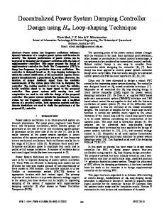
The generic system model used for control of the TSSC.
G2
Fig. 2.
III. T EST SYSTEMS Two different test systems are used to study the performance of the proposed controller. A four-machine system shown in Fig. 2 and a 23-machine system shown in Fig. 3. The fourmachine system is based on a commonly used 230 kV/60 Hz system for studies of inter-area oscillations [9]. Some changes are made from the original system: one tie line is added and the length of the lines interconnecting the two grid areas is stretched to 300 km. Shunt compensation in node 8 is also inserted to maintain a good voltage profile. The generators are equipped with fast exciters and PSS units with an intentionally selected low gain in order to give a system with a small positive damping ratio. The test system has two local power oscillation modes with a frequency in the range of 1 Hz with a reasonable damping and one inter-area mode of oscillation with a frequency in the range of 0.6 Hz which is poorly damped. One important goal for the TSSC in this system is to improve the damping of the inter-area mode. The 23-machine system is the Nordic 32 system built to model the dynamics of the Nordic power system [10]. This system is in its original form well-damped, mainly because
3
G3
G4
The four-machine test system.
II. G ENERIC SYSTEM MODEL In order to design a POD controller, a system model is required. The nature of inter-area oscillations is often such that there is a dominant mode of oscillation which is significantly less damped than all other modes. With this in mind, a simple way to reduce the total power grid is to view it as a system split into two grid areas and the reactances of the lines interconnecting the areas [8] as seen in Fig. 1. Here, each area is represented by a single synchronous machine with a lumped moment of inertia. In this work, the model parameters are estimated continuously by the controller as the Controlled Series Compensator (CSC) reactance changes using the locally measured responses in the active power (𝑃𝑋 ) of the CSC line. This line is represented by a variable, known reactance 𝑋, which is the sum of the uncompensated line reactance 𝑋0 and the controlled CSC reactance 𝑋𝐶𝑆𝐶 . The model is characterized by four additional parameters: one series reactance 𝑋𝑖 , one parallel reactance 𝑋𝑒𝑞 , the frequency of the interarea oscillation 𝑓𝑜𝑠𝑐 , and its damping exponent 𝜎 assuming the oscillation to be of the form 𝑃 (𝑡) = 𝑒𝜎𝑡 𝑠𝑖𝑛(2𝜋𝑓𝑜𝑠𝑐 𝑡). The inner voltages of the machines are described by voltage phasors of magnitudes 𝐸1,2 and phase angles 𝛿1,2 while the terminal voltages of the machines are assumed to be well controlled by AVR and described by voltage phasors of constant magnitudes 𝑈1,2 and variable phase angles 𝜃1,2 . The ′ ′ transient reactances of the machines are denoted 𝑋𝑑1 and 𝑋𝑑2 .
2
4071
4011
1013
1012
External 4072 1021
1011
4012
4021
North 1022
2032
1014
TSSC
2031
4022 4031
4032 4042
4041 4061
4044 Central 41 1043 1044
61 SouthWest 4062
63
Fig. 3.
43 1042
46
1041 1045 4045
4063
62
42 4046
4043
4051
4047 51
47
The 23-machine test system - Nordic 32.
of well tuned PSS units connected to the system generators. A discussion of the original system characteristics is found in [11]. The loads in the original system are modeled using voltage and frequency dependent load models. To challenge the damping controller, all of the PSS units used in the system were disconnected and the load characteristics were changed to voltage independent loads at nodes 2031 and 2032, and voltage and frequency independent loads at nodes 41, 42, 43, 46, and 51. The system was studied in the normal load case (lf029) and the peak load case (lf028) described in [10]. In the peak load case, the system has the least damped modes: 𝜎1 =0.016, 𝑓1 =0.50 Hz ; 𝜎2 =-0.21, 𝑓2 =0.74 Hz; 𝜎3 =-0.24, 𝑓3 = 0.88 Hz, whereas in the normal load case the least damped modes are 𝜎1 =-0.09, 𝑓1 =0.54 Hz; 𝜎2 =-0.21, 𝑓2 =0.73 Hz; 𝜎3 =-0.27, 𝑓3 =0.89 Hz. The least damped, critical mode, corresponds to the generators in Finland (4071, 4072) and the northern part of Sweden (4011, 4012, 1012, 1013, 1014, 1021, and 1022) swinging towards the rest of the system. To improve the damping of this mode, improve the transient stability in the system, and to control the power flows in the system, a TSSC device is placed in series with the line 4011-4021 where the observability and controllability of the critical mode is good. IV. P RINCIPLES OF POWER OSCILLATION DAMPING Consider an ideal CSC located on one of the tie-lines N8N9 in the four-machine test system. Fig. 4 shows the result of a time-domain simulation of a step change in the CSC
ACCEPTED FOR PUBLICATION IN IEEE TRANSACTIONS ON POWER SYSTEMS, VOL. 25, NO. 1, FEBRUARY 2010
700
800
600
700
3
300 200 100
Power on parallel lines N8−N9 Series compensation level of CSC
0 0
2
4
6
8
100 50 0 10
500 400 300 Power on parallel lines N8−N9 200 100 0 0
Time(s)
Fig. 4. Four-machine system: Power on the CSC line, sum of the power transmitted on the two lines N8-N9 parallel to the CSC line, total power transmitted N8-N9, and level of compensation of the CSC line showing a step change in the CSC reactance at t=3.7 s.
CSC line power 100 Series compensation level of CSC 50 0 2 4 6 8 10 Time(s)
CSC Degree of Compensation (%)
CSC line power
400
600 Power (MW)
Power (MW)
500 Total power N8−N9
CSC Degree of Compensation (%)
Total power N8−N9
Fig. 5. Four-machine system: Power on the CSC line, sum of the power transmitted on the two lines N8-N9 parallel to the CSC line, and total power transmitted N8-N9 after a three-phase fault at N8 - No supplementary damping. 800 700
Power (MW)
Ptotp
500 400
CSC line power
300 PXav 200
Power on parallel lines N8−N9 P
100
Xp
0 0
2
100 Series compensation level of CSC 50 0 4 6 8 10 Time(s)
CSC Degree of Compensation (%)
Total power N8−N9
Ptot0 600
Fig. 6. Four-machine system: Power on the CSC line, sum of the power transmitted on the two lines N8-N9 parallel to the CSC line, total power transmitted N8-N9, and level of compensation of the CSC line after a threephase fault at N8 - Oscillation damping in one step.
800 700
Ptotp
500
Power on parallel lines N8−N9
400 300 PXav 200
CSC line power
100 0 0
P
Series compensation level of CSC
Xp
2
4
6
8
100 50 0 10
CSC Degree of Compensation (%)
Total power N8−N9
Ptot0 600 Power (MW)
reactance when the system is initially in steady-state. It can be seen that an inter-area oscillation is generated as a result of the action of the CSC. If a three-phase to ground fault at node 8 is simulated at t=1.0 s and cleared after 100 ms with no line disconnection and no action of the CSC, a poorly damped inter-area oscillation is established as shown in Fig. 5. Figures 4 and 5 raise the question if it is possible to act with the CSC such that an oscillation in anti-phase of the one caused by the fault is generated. This would then cancel out the oscillation in Fig. 5 totally by a single step change in the reactance. Fig. 6 shows that this is indeed possible. If the controller is limited to act only at times coinciding with the high and low peaks of the oscillation it is theoretically possible to cancel out the oscillation at any given peak. However, Fig. 6 also shows that a very large change in the level of compensation is necessary to fulfill the requirement resulting in a very high level of the power transmitted on the CSC line. In order to find a practical use of this principle, it is necessary to extend it to a two-step practice. Fig. 7 shows this procedure. Here, the controller acts twice on consecutive peaks in the power oscillation which results in an almost total cancellation of the inter-area oscillation. With this technique, it is possible to control the final power on the line with the CSC since the first step in the sequence can be chosen with an optional magnitude, whereas the second step can always cancel the oscillation according to the single-step argument above. Now, what remains is to find a way to determine the necessary step magnitudes of the CSC action to fulfil the requirements. This problem is solved assuming that the grid can be accurately modeled by the generic system model in Fig. 1. First, in order to solve the problem of oscillation cancellation in one step, consider the differential equations describing the model:
Time(s)
𝑑 2 𝛿1 𝑑𝑡2
=
𝜔0 2𝐻1
𝑑2 𝛿2 𝑑𝑡2
=
𝜔0 2𝐻2
( 𝑃𝑚1 −
𝑈1 𝑈2 sin(𝜃1 −𝜃2 ) 𝑋𝑡𝑜𝑡
−
𝐾𝑑1 𝑑𝛿1 𝜔0 𝑑𝑡
𝑃𝑚2 −
𝑈1 𝑈2 sin(𝜃2 −𝜃1 ) 𝑋𝑡𝑜𝑡
−
𝐾𝑑2 𝑑𝛿2 𝜔0 𝑑𝑡
(
) (1) ) .
(2)
Fig. 7. Four-machine system: Power on the CSC line, sum of the power transmitted on the two lines N8-N9 parallel to the CSC line, total power transmitted N8-N9, and level of compensation of the CSC line after a threephase fault at N8 - Oscillation damping and power flow control in two steps.
ACCEPTED FOR PUBLICATION IN IEEE TRANSACTIONS ON POWER SYSTEMS, VOL. 25, NO. 1, FEBRUARY 2010
Here, 𝜔0 denotes the electrical angular frequency of the system, 𝐻1 and 𝐻2 are the constants of inertia of the reduced machine representations of the grid areas, 𝐾𝑑1 and 𝐾𝑑2 are the damping factors of each machine while 𝑃𝑚1 and 𝑃𝑚2 denote the excess mechanical power in each area. The excess mechanical power is defined as the power generated in each area which is not consumed by loads in the same area. The total reactance between the grid areas is denoted 𝑋𝑋𝑒𝑞 𝑋𝑡𝑜𝑡 = 𝑋𝑖 + . (3) 𝑋 + 𝑋𝑒𝑞 When deriving (1) and (2) it was assumed that the power loss in the each machine can be neglected. The units of the parameters are: 𝛿 [rad], 𝑡 [s], 𝐻 [s], 𝜃 [rad], 𝜔 [rad/s], 𝑃𝑚 [p.u.], 𝐸 [p.u.], 𝑈 [p.u.], 𝑋𝑡𝑜𝑡 [p.u.] and 𝐾𝑑 [p.u. torque/p.u. speed]. Now, assume that the angle differences, 𝛿1 − 𝜃1 and 𝛿2 − 𝜃2 , are small in magnitude compared to the magnitude of the phase angle difference 𝜃1 − 𝜃2 between the machines. This is true if ′ ′ 𝑋𝑑1 ≪ 𝑋𝑡𝑜𝑡 and 𝑋𝑑2 ≪ 𝑋𝑡𝑜𝑡 . At the positive and negative peaks of the power oscillation, the difference 𝜃1 − 𝜃2 assumes its highest and lowest values and the time-derivatives of 𝜃1 and 𝜃2 are both zero. Since only one mode of power oscillations exists in the considered system, the time-derivatives of 𝛿1 and 𝛿2 can also be assumed to be zero at these instants. In order to stabilize the system at one of these instants in time, it is necessary to also force the second time-derivative of 𝛿1 and 𝛿2 to be zero. If this is done, all higher order derivatives of 𝛿1 and 𝛿2 will also be zero and no inter-area oscillations will longer occur in the system. This can be achieved by assuring that the right-hand sides of both (1) and (2) are zero. In order to illustrate the damping process, the situation in Fig. 6 is used as an example. The value of 𝑃𝑚1 = −𝑃𝑚2 = 𝑃𝑡𝑜𝑡0 which is assumed to be constant during the change in the CSC reactance is estimated immediately before the controller operation as indicated in Fig. 6. This is done with the knowledge of the grid parameters 𝑋 and 𝑋𝑒𝑞 by measuring the average power (calculated over one oscillation cycle) on the line with the CSC, 𝑃𝑋𝑎𝑣 and applying 𝑋𝑒𝑞 + 𝑋 𝑃𝑡𝑜𝑡0 = 𝑃𝑋𝑎𝑣 . (4) 𝑋𝑒𝑞 Eq. (4) is also valid for instantaneous values of the line power 𝑃𝑋 and the total power 𝑃𝑡𝑜𝑡 . In order to force the right-hand sides of (1) and (2) to zero at the instant t=3.7 s when the power oscillation on the line has a negative peak, assume that the angle difference 𝜃1 −𝜃2 does not change during the change in reactance and that the terminal voltages of the generators are constant. This can be motivated since the angle differences 𝛿1 −𝜃1 and 𝛿2 −𝜃2 are small and the rotor angles 𝛿1 and 𝛿2 are governed by inertia and move only with a large time constant. In this case, the product 𝑈1 𝑈2 sin(𝜃1 − 𝜃2 ), valid both before and after the reactance step can be calculated in terms of the initial power and reactance values. This yields ′ 𝑃𝑡𝑜𝑡 =
𝑃𝑡𝑜𝑡𝑝 𝑋𝑡𝑜𝑡 𝑈1 𝑈2 sin(𝜃1 − 𝜃2 ) = . ′ ′ 𝑋𝑡𝑜𝑡 𝑋𝑡𝑜𝑡
(5)
Here, the total instantaneous power transmitted between the ′ areas before and after the step is denoted 𝑃𝑡𝑜𝑡𝑝 and 𝑃𝑡𝑜𝑡
4
respectively, and the total reactance according to (3) initially ′ and finally is given as 𝑋𝑡𝑜𝑡 and 𝑋𝑡𝑜𝑡 respectively. 𝑃𝑡𝑜𝑡𝑝 is found by measuring the power on the CSC line at the peak of the oscillation, 𝑃𝑋𝑝 as indicated in Fig. 6 and applying (4). ′ ′ If 𝑃𝑡𝑜𝑡 is forced to be equal to 𝑃𝑡𝑜𝑡0 by choosing 𝑋𝑡𝑜𝑡 in a suitable way, the right hand sides of (1) and (2) will be zero since the time-derivatives of 𝛿1 and 𝛿2 are already zero at this instant. The ratio of the total reactance before and after the reactance change required for this can be found by setting (5) equal to 𝑃𝑡𝑜𝑡0 . Thus, 𝑃𝑡𝑜𝑡0 𝑋𝑡𝑜𝑡 = . ′ 𝑋𝑡𝑜𝑡 𝑃𝑡𝑜𝑡𝑝
(6)
The required change in the total reactance can now be expressed as ( ) 𝑃𝑡𝑜𝑡𝑝 ′ Δ𝑋𝑡𝑜𝑡 = 𝑋𝑡𝑜𝑡 − 𝑋𝑡𝑜𝑡 = − 1 𝑋𝑡𝑜𝑡 (7) 𝑃𝑡𝑜𝑡0 and the required change in the initial CSC line reactance 𝑋0 is found by applying (3) to the situation before and after the reactance change. This gives the non-linear control law Δ𝑋 =
Δ𝑋𝑡𝑜𝑡 (𝑋0 + 𝑋𝑒𝑞 )2 . 2 − Δ𝑋 𝑋 − Δ𝑋 𝑋 𝑋𝑒𝑞 𝑡𝑜𝑡 0 𝑡𝑜𝑡 𝑒𝑞
(8)
In order to solve the combined damping and power flow problem in two steps, it is assumed that the total reactance according to (3) before the first reactance step is 𝑋𝑡𝑜𝑡0 , after the first step 𝑋𝑡𝑜𝑡1 , and after the second step 𝑋𝑡𝑜𝑡2 . The effective reactance of the CSC line is denoted 𝑋0 initially, 𝑋1 following the first step, and 𝑋2 after the second step. It can be immediately recognized that the final compensation state given by 𝑋2 can be calculated since it is assumed that the initial average power on the line is known as 𝑃𝑋𝑎𝑣 as in the single-step case above and the desired set-point of the average power flow is denoted 𝑃𝑋𝑠𝑝 . The expression becomes ( ) 𝑋𝑒𝑞 + 𝑋0 𝑃𝑋𝑠𝑝 = 𝑃𝑋𝑎𝑣 (9) 𝑋𝑒𝑞 + 𝑋2 by current sharing of the parallel lines in the circuit assuming that the average transmitted total power is constant during the procedure (see [8]). By means of (3), 𝑋𝑡𝑜𝑡2 is then known. To calculate 𝑋𝑡𝑜𝑡1 , denote the instantaneous total power transmitted between the areas before the steps at the point where the controller starts to act as 𝑃𝑡𝑜𝑡𝑝 , the total power after the first step as 𝑃𝑝1 , and the total power right before the ′ second step as 𝑃𝑝1 . From (5) it is now found that: 𝑃𝑡𝑜𝑡𝑝 𝑋𝑡𝑜𝑡0 = 𝑃𝑝1 𝑋𝑡𝑜𝑡1 .
(10)
The value of the total power right before the second step can be approximated by recognizing that the total power always oscillates around its average value 𝑃𝑡𝑜𝑡0 , ′ 𝑃𝑝1 = (𝑃𝑡𝑜𝑡0 − 𝑃𝑝1 )𝑒𝜎𝑇𝑜𝑠𝑐 /2 + 𝑃𝑡𝑜𝑡0 .
(11)
Here it has been assumed that the power oscillation can be described by a sine function in time. The real part of the eigenvalue corresponding to the inter-area mode is given as 𝜎 and 𝑇𝑜𝑠𝑐 is the cycle time of the oscillation. Since it is known
ACCEPTED FOR PUBLICATION IN IEEE TRANSACTIONS ON POWER SYSTEMS, VOL. 25, NO. 1, FEBRUARY 2010
that the second reactance step must cancel the oscillation completely, the second reactance step must fulfil ′ 𝑃𝑝1 𝑋𝑡𝑜𝑡1 = 𝑃𝑡𝑜𝑡0 𝑋𝑡𝑜𝑡2
(12)
and bring the instantaneous total power value to equal the average level 𝑃𝑡𝑜𝑡0 . Combining (10), (11), and (12) now yields ) (( ) 𝑃𝑡𝑜𝑡𝑝 𝑋𝑡𝑜𝑡0 𝑃𝑡𝑜𝑡0 − 𝑒𝜎𝑇𝑜𝑠𝑐 /2 + 𝑃𝑡𝑜𝑡0 𝑋𝑡𝑜𝑡1 (13) 𝑋𝑡𝑜𝑡1 = 𝑃𝑡𝑜𝑡0 𝑋𝑡𝑜𝑡2 . Thus, the reactance 𝑋𝑡𝑜𝑡1 can be calculated, using (4) to calculate 𝑃𝑡𝑜𝑡𝑝 and 𝑃𝑡𝑜𝑡0 from the measured values of the peak power 𝑃𝑥𝑝 and the average power 𝑃𝑋𝑎𝑣 indicated in Fig. 7. By means of (3) and (13), 𝑋1 is now known and since 𝑋0 is known initially and 𝑋2 has been calculated, the control law is complete and the necessary reactance changes can be calculated as Δ𝑋1 = 𝑋1 − 𝑋0 and Δ𝑋2 = 𝑋2 − 𝑋1 . The damping and power flow control methods proposed here are believed to be original work even though discrete, timeoptimal methods for damping of power oscillations by means of CSC have been described before [13], [14], [15]. V. E STIMATION OF THE SYSTEM MODEL PARAMETERS In this work, the controller is designed based on a generic system model. This means that the model parameters must be estimated to fit the current situation in the grid in order for the controller to be successful. Since a typical power grid is far more complex than the system model and due to the physical limitations of the CSC device, the real controller will never work in the ideal way which is described in the previous section. Instead, the two-step control law will have to be reapplied until the power oscillation is canceled out. The controller is time-discrete in nature which enables the parameter estimation routines to be developed based on the open-loop step response of the reduced system in Fig. 1 to changes in the CSC reactance. In [16], the equations governing the step response of the system when it is initially subject to an electro-mechanical oscillation are derived assuming that the CSC is ideal. The relations between the initial instantaneous value of the power on the CSC line, 𝑃𝑋 and the instantaneous ′ value of the same line power after the step 𝑃𝑋 as well as the average values (calculated over one oscillation cycle) of the ′ CSC line power before and after the step, 𝑃𝑋𝑎𝑣 and 𝑃𝑋𝑎𝑣 respectively are derived as ( ) 𝑋𝑒𝑞 + 𝑋 ′ 𝑃𝑋𝑎𝑣 (𝑋) = 𝑃𝑋𝑎𝑣 , (14) 𝑋𝑒𝑞 + 𝑋 ′ ′ 𝑃𝑋 = 𝑃𝑋
(𝑋 + 𝑋𝑒𝑞 ) 𝑋𝑡𝑜𝑡 ′ . (𝑋 ′ + 𝑋𝑒𝑞 ) 𝑋𝑡𝑜𝑡
(15)
Here, 𝑋 and 𝑋 ′ denote the initial and final values of the CSC ′ line reactance, and 𝑋𝑡𝑜𝑡 and 𝑋𝑡𝑜𝑡 denote the initial and final values of the total reactance. These relations can be directly applied to derive non-linear estimation relations for the grid parameters 𝑋𝑖 and 𝑋𝑒𝑞 . These are used to estimate the grid parameters based on the measured instantaneous and average values of the line power of the line where the CSC is placed
5
before and after each new step during the CSC operation and the known values of the apparent CSC line reactance before and after the reactance step. In the implementation of the controller, consecutive estimates of the system parameters are averaged in order to give a more robust performance. One motivation for using a non-linear estimation technique instead of a linear one such as a Recursive Least Squares (RLS) algorithm is that the damping control law is non-linear which may lead to large deviations from the linearization point of the system equations, which in turn may lead to errors in the linear estimation. VI. P RINCIPLES OF TRANSIENT STABILITY IMPROVEMENT In this work, an open-loop strategy is used to improve the transient stability. The background of the strategy is given in [17]. The goal is to maximize the transient stability of the system when a fault which threatens the stability is detected. The scheme is enabled directly when the fault is detected and acts in two stages during the first-swing of the generator angles. It can (after it has been initiated) be concluded in the following compact form: 𝑋𝐶𝑆𝐶 = 𝑋𝐶𝑆𝐶𝑚𝑖𝑛 , (𝜃˙𝑠 − 𝜃˙𝑟 ) > 0
(16)
𝑋𝐶𝑆𝐶 = 𝑋𝐶𝑆𝐶𝑚𝑖𝑛 , (𝜃˙𝑠 − 𝜃˙𝑟 ) < 0, (𝜃𝑠 − 𝜃𝑟 ) > 90∘ (17) 𝑋𝐶𝑆𝐶 = 𝑐𝑋𝐶𝑆𝐶𝑚𝑖𝑛 ,
(18)
(𝜃˙𝑠 − 𝜃˙𝑟 ) < 0, (𝜃𝑠 − 𝜃𝑟 ) < 90∘ , 𝑐 ∈ [0, 1]. Here, the electrical angles of the reduced machine equivalents in the sending and receiving area of Fig. 1 are denoted 𝜃𝑠 and 𝜃𝑟 respectively, and the minimum value of the CSC reactance (maximum amount of compensation) is given as 𝑋𝐶𝑆𝐶𝑚𝑖𝑛 . The scheme selects the maximum compensation level at fault clearance and reverts to a lower level of series compensation as the angle difference declines after the first swing. The switching instant of the scheme is determined from the local signals at the TSSC location in a manner described in [16]. Following the transient control scheme operation in two steps described above, the damping controller is commonly initiated. Even if the system is transiently stable and survives the first swing, provided that the pre-programmed scheme is used, the system may still exhibit transient instability if the series compensation level is significantly reduced during one of the subsequent swings. In order to maximize the transient stability during subsequent swings, the controller is required to maintain the maximum possible degree of compensation when the angle separation 𝜃𝑠 − 𝜃𝑟 is increasing. To achieve this goal without exceeding the short-term overload limit of the CSC line, the transient controller alters the set-point of the power flow control function which is included in the POD controller. The set-point 𝑃𝑋𝑠𝑝 is changed such that it equals the short-term overload limit 𝑃𝑙𝑖𝑚𝑖𝑡 . A conservative choice of 𝑃𝑙𝑖𝑚𝑖𝑡 is the active power level on the CSC line which can be allowed for the time it takes for the Transmission System Operator (TSO) to re-dispatch the system to comply with the N-1 criterion of the new conditions (15-30 min).
ACCEPTED FOR PUBLICATION IN IEEE TRANSACTIONS ON POWER SYSTEMS, VOL. 25, NO. 1, FEBRUARY 2010
The transient capability can be further improved if the system allows 𝑃𝑋𝑠𝑝 to be chosen higher than the thermal limit during the time when the damping controller is active after a fault. An even larger improvement of the transient stability can be achieved if the operating range of the CSC is limited during the damping event. In this case, a maximum limit of 𝑋𝐶𝑆𝐶 , 𝑋𝐶𝑆𝐶𝑙𝑖𝑚 other than the physical limit of the device can be set when the transient scheme is triggered. For example, it may be coherent to choose 𝑋𝐶𝑆𝐶𝑙𝑖𝑚 = 𝑐𝑋𝐶𝑆𝐶𝑚𝑖𝑛 such that 𝑋𝐶𝑆𝐶𝑚𝑖𝑛 ≤ 𝑋𝐶𝑆𝐶 ≤ 𝑐𝑋𝐶𝑆𝐶𝑚𝑖𝑛 , ensuring the same minimum level of compensation of the CSC device during the whole controller operation. This reduces the risk of transient instability even though limiting the operating range of the device decreases the effectiveness of the damping controller which makes the method a trade-off between transient stability improvement and oscillation damping enhancement. Detection of faults threatening the transient stability of the system is not addressed in this work. However, a comprehensive literature study of the research on on-line transient stability assessment is found in [18]. In the simulations presented in this paper it has been assumed that the transient control scheme is triggered at clearance of all the studied faults, regardless of their severity. In the less severe faults, this may give a somewhat less effective damping of the power oscillation, while the scheme is essential for the transient stability of the severe faults. A similar transient stability improvement strategy as the one proposed here is described for a shuntconnected FACTS device in [19]. VII. T HE COMPLETE CONTROLLER A block diagram of the controller and TSSC models is shown in Fig. 8. The controller utilizes only locally measured quantities measured at the TSSC location. Generally, a fault in the system first leads to a risk of transient instability which initiates the transient controller. When this controller has performed its sequence there is commonly a power oscillation in the system which is detected by an RLS algorithm [20]. The RLS algorithm is based on the assumption that the line power is composed of a zero frequency component (the average value) and a component which has a known frequency range (the dominant power oscillation frequency). The algorithm utilizes an expected oscillation frequency when no oscillations are at hand. At any event that causes power oscillations, the frequency parameter is adapted to the actual oscillation frequency by a PI-controller. The algorithm gives a realtime estimation of the average line power (𝑃𝑋𝑎𝑣 ), oscillation amplitude (𝑃𝑋𝑜𝑠𝑐 ), frequency (𝑓𝑜𝑠𝑐 ), and phase (𝜑𝑜𝑠𝑐 ). The RLS algorithm is necessary in order to determine the input and timing for the damping controller and the parameter estimator. The bandwidth of the RLS algorithm is determined by the demands of the controller which state that it is necessary to gain information of the oscillation phase and amplitude as well as the average value of the line power within one half of a power oscillation cycle after a step in the TSSC reactance. A higher bandwidth naturally means faster response but also a larger sensitivity to noise. The RLS estimator used here has been tested with a noise level of 1% of the input signal with good results.
PI controller fosc -tuner
System Identification
Xi & Xeq RLS estimation
Pav Posc f osc
Fig. 8.
POD / fast power flow controller
PXsp IX
PX
6
Transient + controller XTR PI - slow XPI power flow Pref controller
XTSSC-max
XPOD XCSC
1 sTTSSC+1
TSSC discretization
XTSSC
XTSSC-min
Block diagram of the TSSC model with the proposed controller.
When an oscillation with an amplitude exceeding a certain level is detected by the RLS algorithm, the damping controller is enabled. The damping controller is based on the control law of damping and power flow control in two time-steps presented in Section IV. Since the damping controller/fast power flow controller is only active when power oscillations are present, a separate slow PI-controller with power reference value 𝑃𝑟𝑒𝑓 is necessary for long-term power flow control. These controllers contribute with the terms 𝑋𝑃 𝑂𝐷 , 𝑋𝑇 𝑅 , and 𝑋𝑃 𝐼 to the desired reactance of the CSC - 𝑋𝐶𝑆𝐶 . All controllers use the active power 𝑃𝑋 of the CSC line or estimations of it as input signals. The transient controller also uses the current magnitude of the CSC line 𝐼𝑋 as an input signal. The focus of this paper is to study the damping and transient control performance of the controller and the long-term PI power flow controller is thus omitted in the implementation. For practical reasons, the TSSC is modeled as a discrete controllable reactance with the dynamics of a first-order low-pass filter of time constant 𝑇𝑇 𝐶𝑆𝐶 = 15 ms. In reality, the delay of a TSSC is variable between zero and 20 ms [21]. This modeling difference is of minor importance, since the power oscillations which are subject to damping have much slower dynamic properties. VIII. R ESULTS AND DISCUSSION A. Four-machine system study Here, a TSSC equipped with the proposed controller was implemented in the four-machine system of Fig. 2 and studied in digital simulations using the software SIMPOW from STRI AB. The system exhibits poorly damped inter-area oscillations with a frequency of about 0.6 Hz when it is subject to a disturbance. The TSSC, which is placed on one of the interconnecting lines N8-N9 to damp the inter-area mode, is selected to consist of three switched series-connected capacitive elements. This arrangement gives the TSSC an operating range where the inserted reactance can be varied in eight discrete equidistant steps between the the minimum reactance 𝑋𝑇 𝐶𝑆𝐶𝑚𝑖𝑛 which was chosen to be -50 % of the initial reactance of the TSSC line and the maximum reactance 𝑋𝑇 𝐶𝑆𝐶𝑚𝑎𝑥 which is zero. The controller performance was studied by simulation of four different contingencies for a high- (200 MW/line) and a low- (60 MW/line) loading situation of the tie lines N7N9 between the grid areas. The loads used for the loading cases (high/low) were 𝑃𝐿7 =967/1367 MW, 𝑄𝐿7 =100/200 Mvar and 𝑃𝐿9 =1967/1367 MW, 𝑄𝐿9 =100/200 Mvar and the active power generation of generators 1 and 2 was 1600 MW in total. Simulated measurement noise with a standard
ACCEPTED FOR PUBLICATION IN IEEE TRANSACTIONS ON POWER SYSTEMS, VOL. 25, NO. 1, FEBRUARY 2010
B C D
A 3-phase short circuit (SC) at node 8 cleared with no line disconnection after 200 ms. A 3-phase SC at node 8 cleared by disconnection of one N8-N9 line in parallel to the CSC after 200 ms. A 3-phase SC at node 8 cleared by disconnecting one of the N7-N8 lines after 200 ms. A load disconnection at node 7: Δ𝑃 =-250 MW Δ𝑄=-50 MVAr.
An example of the controller performance in fault B for the high-load case is given in Figures 9, 10, and 11. The results of all the studied cases are concluded in Table I. From Fig. 9, it can be seen that the transient controller is activated at fault clearance at t=1.2 s and disengaged at t=1.7 s. The damping controller is engaged at t=2.3 s. At first, the grid parameters are unknown and the parameters are reset to a safe state. As the system parameters are estimated with better accuracy, the damping is gradually more effective. The damping of the oscillation is completed at t=5.5 s and the power flow on the line is stabilized close to the set-point 350 MW which is assumed to be the short-term overload limit of the line in this case. In most of the studied cases, this power flow target cannot be reached and the TSSC reactance saturates at its maximum capacitive value following the damping event. In Fig. 10, the terminal voltage magnitude and phase angle in phase A of G2 and G4 are plotted. Here, the damping effect of the controller on the generator angles is clearly seen. Fig. 10 also shows the influence of the reactance steps of the TSSC on the generator terminal voltages. Since the assumptions of the controller are that the generator terminal voltages and phase angles are piece-wise constant during each reactance step, the variations seen from Fig. 10 will influence the stability of the controller. This issue will be discussed in Section VIII-C. Fig. 11 shows the evolution of the system model parameters 𝑋𝑖 , 𝑋𝑒𝑞 , and 𝑓𝑜𝑠𝑐 in fault B for the high-load case. The system exhibits a dominant inter-area mode of oscillation in the range of 0.51-0.74 Hz depending on configuration. The initial guess of 𝑓𝑜𝑠𝑐 is chosen to be 0.6 Hz. The parameters 𝑋𝑖 and 𝑋𝑒𝑞 are updated whenever a reactance step response in the power of the TSSC line above a certain magnitude is detected. It can be seen that the parameters stabilize close to 𝑋𝑖 =0.17 p.u. and 𝑋𝑒𝑞 =0.15 p.u. on a 100 MW, 230 kV base after a few time-steps. The estimated value of 𝑋𝑒𝑞 is close to what could be expected judging from the line length and inductive reactance characteristics of the remaining line N8N9 in parallel to the TSSC line. The estimated value of 𝑋𝑖 is somewhat higher than what could be expected from the line characteristics. This is a general pattern which is seen in most simulation cases. The reason for this may be the simplicity of the system model which causes various un-modeled dynamics of the generators and AVR to be included in the 𝑋𝑖 parameter. The PI-controller tuning 𝑓𝑜𝑠𝑐 is continuously active as long as the power oscillation exceeds 15 MW in amplitude. It is
Pline, controller enabled kTSSC, controller enabled
500
P
, controller disabled
line
400
300 70 200
55 40
100
0 0
Degree of compensation (%)
A
600
Active power (MW)
deviation of 1 % of the input signal value was added to the controller input. All loads were modeled as voltage dependent with constant current characteristics for the active power and constant impedance characteristics for the reactive power load. The studied fault cases were:
7
25
2
4
6
8
10 0 10
Time (s)
Fig. 9. Four-machine system, 600 MW inter-area power transfer, fault B: CSC line power (𝑃𝑙𝑖𝑛𝑒 ) and series compensation level (𝑘𝑇 𝑆𝑆𝐶 ), TSSC controller enabled/disabled.
judged difficult to continuously estimate the damping exponent 𝜎 in a reliable manner. Thus, this parameter is set to zero. Since power systems are rarely operated such that negative damping of power oscillations is likely, this is a worst case assumption. This means that the controller will be based on a correct assumption in the worst case where it is needed the most. If negative damping can be expected, 𝜎 can be set to a positive value ensuring optimal performance in the worst case on the expense of the performance in non-critical conditions. The results of the studied fault cases are concluded in Fig. 12 and Table I. Fig. 12 shows the amplitudes of the total inter-area power oscillation in the four high power transfer cases as a function of time measured by an RLS phasor estimator implemented in the simulator. It can be seen that the improvement of the system damping is substantial when the proposed controller is used. In Table I, the maximum amplitude of the total power oscillation is given as Δ𝑃𝑜𝑠𝑐 (MW) and the damping ratios with the damping controller disengaged and engaged are given as 𝜁𝑖 and 𝜁𝑇 𝑆𝑆𝐶 respectively. 𝜁𝑖 is the small-signal value for the post-fault system with no controller while 𝜁𝑇 𝑆𝑆𝐶 is a value calculated for comparison from the time-domain simulations with the controller. The value is obtained by studying the amplitude of the total power oscillation initially and after the damping event. These two values are then fitted to a decaying exponential curve and the equivalent damping ratio is thus calculated. This is done since the controller is adaptive and the small-signal value of the oscillation eigenvalue does not take into account the adaptive merits of the controller. The post-fault frequency of the system eigenvalue corresponding to the inter-area mode is given as 𝑓𝑜𝑠𝑐 for each case. The required time after fault clearance for the power oscillation amplitude to settle below 5 MW in the time-domain simulation is given for each fault for the undamped system as 𝑇𝑖 (s) and for the damped system as 𝑇𝑇 𝑆𝑆𝐶 (s). It can be seen from Table I that the damping of the inter-area oscillation mode is significantly improved to satisfactory values in all of the studied cases.
ACCEPTED FOR PUBLICATION IN IEEE TRANSACTIONS ON POWER SYSTEMS, VOL. 25, NO. 1, FEBRUARY 2010
UaG2nc
1.02
UaG4nc Ua
1
G2c
Ua
G4c
0.98 0
2
4
6
8
Angle (deg.)
80
θ
60
θG2c−θG4c
G2nc
−θ
G4nc
40 20 2
4
6
300
case A case B case C case D
200 100 0 0
5
10
Time (s) (b)
0 0
Osc. amplitude (MW)
1.04
(a) 300
Osc. amplitude (MW)
Voltage (p.u.)
(a)
8
8
10 Time(s) (b)
15
case A case B case C case D
200 100 0 0
20
5
10
10 Time(s)
15
20
Time (s)
Fig. 10. Four-machine system, 600 MW inter-area power transfer, fault B: (a) Terminal voltages in phase A of generators G2 and G4 with the controller enabled (𝑈 𝑎𝐺2𝑐 , 𝑈 𝑎𝐺4𝑐 ) and disabled (𝑈 𝑎𝐺2𝑛𝑐 , 𝑈 𝑎𝐺4𝑛𝑐 ), (b) Generator terminal voltage phase differences between G2 and G4 with the controller enabled (𝜃𝐺2𝑐 − 𝜃𝐺2𝑐 ) and disabled (𝜃𝐺2𝑛𝑐 − 𝜃𝐺2𝑛𝑐 ).
0.44 Xeq
0.4
fosc X
i
0.3
0.64
Frequency (Hz)
Reactance (p. u.)
0.35
0.69
0.25 0.2
0.59
0.15 0.1
0.54
0.05 0 0
2
4
6
8
0.49 10
Time (s)
Fig. 11. Four-machine system, 600 MW inter-area power transfer, fault B: Estimated system model parameters 𝑋𝑖 , 𝑋𝑒𝑞 , and 𝑓𝑜𝑠𝑐 , TSSC controller enabled.
Fig. 12. Four-machine system, 600 MW inter-area transfer: Total oscillation amplitudes for case A (solid), case B (dashed), case C (dash-dot), and case D (dotted) with TSSC controller disabled (a) and enabled (b).
B. 23-machine system study In order to test the CSC controller in a more realistic power system, the controller was implemented with a TSSC placed in the Nordic 32 system as shown in Fig. 3. In this system, the Southwest and the External areas are essentially self-supporting while the Central region imports half of its power consumption from the Northern area. Here, the goal for the CSC controller was to improve the damping of the critical inter-area oscillation mode where the External and North regions oscillate with the rest of the system. The mode has an oscillation frequency of approximately 0.5 Hz. Mode shapes of the least damped modes of the Nordic 32 system can be found in [11]. The system was studied using SIMPOW in time-domain simulations of four different severe contingencies at two different power flow levels of the North-Central intertie. In the normal load flow case (lf029 in [10]) the power transfer between North and Central is about 2800 MW and in the peak load flow case (lf028 in [10]) about 3300 MW is transferred between the regions. The studied faults were: A B
TABLE I S IMULATION RESULTS OF THE FOUR - MACHINE SYSTEM , FAULTS A-D FOR INTER - AREA POWER TRANSFERS OF 180 MW AND 600 MW.
600 MW
180 MW
𝑓𝑜𝑠𝑐 𝜁𝑖 Δ𝑃𝑜𝑠𝑐 𝜁𝑇 𝑆𝑆𝐶 𝑇𝑖 𝑇𝑇 𝑆𝑆𝐶 𝑓𝑜𝑠𝑐 𝜁𝑖 Δ𝑃𝑜𝑠𝑐 𝜁𝑇 𝑆𝑆𝐶 𝑇𝑖 𝑇𝑇 𝑆𝑆𝐶
A 0.67𝐻𝑧 0.071% 210𝑀 𝑊 8.3% 720𝑠 8.2𝑠 0.73𝐻𝑧 1.4% 110𝑀 𝑊 7.3% 30𝑠 7.4𝑠
B 0.54𝐻𝑧 1.9% 160𝑀 𝑊 17% 56𝑠 5.6𝑠 0.68𝐻𝑧 1.7% 100𝑀 𝑊 15% 33𝑠 5.3𝑠
C 0.51𝐻𝑧 2.7% 150𝑀 𝑊 8.8% 33𝑠 9.6𝑠 0.68𝐻𝑧 1.9% 110𝑀 𝑊 9.3% 26𝑠 6.9𝑠
D 0.68𝐻𝑧 1.3% 60𝑀 𝑊 21% 27𝑠 2.3𝑠 0.74𝐻𝑧 2.8% 40𝑀 𝑊 13% 14𝑠 5.3𝑠
C D
A 3-phase short circuit at node 4011 for 100 cleared by disconnection of the line 4011-4012. A 3-phase short circuit at node 4011 for 100 cleared by disconnection of the line 4011-4022. A 3-phase short circuit at node 4012 for 100 cleared by disconnection of the line 4012-4022. A 3-phase short circuit at node 4041 for 100 cleared by disconnection of the line 4031-4041.
ms ms ms ms
The TSSC was selected to consist of four series-connected capacitive elements each equipped with a parallel bipolar switch. This gives the TSSC an operating range where the inserted reactance can be varied in 16 discrete equidistant steps between the minimum reactance 𝑋𝑇 𝐶𝑆𝐶𝑚𝑖𝑛 which was chosen to be -70 % of the initial CSC line reactance and the maximum reactance 𝑋𝑇 𝐶𝑆𝐶𝑚𝑎𝑥 which is zero. The TSSC was installed on line 4011-4021 close to node 4011 where the observability and controllability of the critical oscillation
ACCEPTED FOR PUBLICATION IN IEEE TRANSACTIONS ON POWER SYSTEMS, VOL. 25, NO. 1, FEBRUARY 2010
9
0.7
0.1
1300
X
1200
600 400
70 P
, controller enabled
line
Pline, controller disabled
200
k 0 0
5
10
15
0.06
0.6
0.04
0.55
0.02
0.5
30
, controller enabled
TSSC
0.65 frequency (Hz)
800
f
osc
Reactance (p.u.)
Active power (MW)
1000
Degree of compensation (%)
i
Xeq
0.08
0
20
Time (s)
0 0
5
10 Time(s)
15
0.45 20
Fig. 13. Twenty-three machine system, normal load case (lf029), fault B: TSSC line power (𝑃𝑙𝑖𝑛𝑒 ) with the TSSC controller enabled/disabled and TSSC degree of compensation (𝑘𝑇 𝑆𝑆𝐶 ) with the controller enabled.
Fig. 14. Twenty-three machine system, normal load case (lf029), fault B: Estimated system model parameters 𝑋𝑖 , 𝑋𝑒𝑞 and 𝑓𝑜𝑠𝑐 , TSSC controller enabled.
mode is high. No simulated measurement noise was used in this study. An example of how the controller operates is shown in Fig. 13 and Fig. 14. Here, fault B is studied in the normal load case. It can be seen that the TSSC controller effectively damps the inter-area oscillations in the system within approximately 7 seconds. The post-fault power flow set-point used by the transient controller was in this study set to 1000 MW, which is a conservative setting close to the thermal overload limit of the line. In this case, the set level cannot be reached and the TSSC saturates at the highest possible compensation level after the event. It can be noted that the transient stability controller fails to determine the instant for the second switching in the openloop scheme during this fault case. This occurs occasionally due to interference of other oscillation modes in the RLS-based detection scheme. This does not degrade the transient stability improvement of the controller but it generally gives a slightly less effective damping of the oscillation mode. The adaptive controller estimates the system parameters according to the generic system model and the evolution of the parameters is shown in Fig. 14. Here, the reactance parameters 𝑋𝑖 and 𝑋𝑒𝑞 are seen to stabilize close to 𝑋𝑖 =0.032 p.u. and 𝑋𝑒𝑞 =0.065 p.u. on a base of 100 MW and 400 kV while the estimation of the oscillation frequency is less stable in the range 0.5-0.6 Hz. It should be noted that the inter-area oscillation frequency is dependent on the level of series compensation in the system. A fixed value should, therefore, not be expected during the time when the damping controller acts. ”True” values of the reactance parameters are not straightforward to calculate but it can be concluded that the estimates are in the right range considering the line reactance characteristics of the system given in [10]. The simulation results of the TSSC controller performance in the different fault cases are shown graphically in Fig. 15, Fig. 16, and compiled in Table II. The amplitude of the total power oscillation across the inter-tie consisting of the lines 4011-4021, 4011-4022, and 4012-4022 in the system was measured with an RLS phasor estimator for the system with the TSSC controller and the uncontrolled system.
This is the narrow power corridor connecting the External and North Regions to the Central region where the TSSC is placed, and the inter-area oscillation is very clearly observable. The results of the simulations are given in Fig. 15 for the normalload case and in Fig. 16 for the peak-load case. During the first few seconds after a fault, the RLS estimation of the oscillation amplitude is not reliable due to the interference with other modes. This is clearly seen in Fig. 15 where the estimated amplitudes show violent variations during the first 3-4 seconds after the fault, but then stabilize to reveal a slowly decaying oscillation amplitude. Fig. 15 (a) shows the situation when no TSSC controller is used and Fig. 15 (b) illustrates the case when the TSSC controller is enabled. It is seen that the controller improves the damping of the inter-area mode significantly for all the studied contingencies. Fig. 16 illustrates the more severe case when the transmitted power between the North and Central regions in the system is increased. Here, it is seen that in the case without damping controller, cases B and C (marked with (1) in the figure) exhibit transient instability while case D (marked (2)) shows oscillatory instability after a few seconds. Case A is stable, but it exhibits a very poor damping of the inter-area mode. When the controller is enabled, the system is stable and the controller shows a good damping performance in all cases except for case C (marked by (3)) which is unstable. In this case, it can be shown that a TSSC controller which limits the reactance operation region of the TSSC after a severe fault is beneficial. If such a controller is used, limiting the degree of compensation of the TSSC to a band between 37 and 70 %, case C can also be stabilized (marked by (4)) provided that the line can sustain a temporary power flow of up to 1200 MW during the time of oscillation damping. In Table II, the data of each simulated fault is given with the same denotations as in Table I. 𝑇𝑖 (s) and 𝑇𝑇 𝑆𝑆𝐶 are here given as the required times after fault clearance for the power oscillation amplitude measured on the TSSC line to settle below 15 MW for the undamped and damped system. The damping ratio of the mode improves slightly with an increased
Osc. amplitude (MW)
Osc. amplitude (MW)
ACCEPTED FOR PUBLICATION IN IEEE TRANSACTIONS ON POWER SYSTEMS, VOL. 25, NO. 1, FEBRUARY 2010
(a) case A case B case C case D
400 200
5
10 Time(s) (b)
15
20
case A case B case C case D
400 200 0 0
5
10 Time(s)
15
20
Osc. amplitude (MW)
Fig. 15. Twenty-three machine system, normal load case (lf029): Total oscillation amplitudes for case A (solid), case B (dashed), case C (dash-dot) and case D (dotted) with the TSSC controller disabled (a) and enabled (b).
Osc. amplitude (MW)
TABLE II S IMULATION RESULTS OF THE TWENTY- THREE MACHINE SYSTEM , FAULTS A-D FOR THE NORMAL AND THE PEAK LOAD CASE .
Peak 0 0
case A case B case C case D
(1) (2)
400 200 0 0
600
5
10 Time(s) (b)
15
(4)
(3)
20
case A case B case C case D
400 200 0 0
5
10 Time(s)
Normal
𝑓𝑜𝑠𝑐 𝜁𝑖 𝜁𝑝𝑜𝑠𝑡 Δ𝑃𝑜𝑠𝑐 𝜁𝑇 𝑆𝑆𝐶 𝑇𝑖 𝑇𝑇 𝑆𝑆𝐶 𝑓𝑜𝑠𝑐 𝜁𝑖 𝜁𝑝𝑜𝑠𝑡 Δ𝑃𝑜𝑠𝑐 𝜁𝑇 𝑆𝑆𝐶 𝑇𝑖 𝑇𝑇 𝑆𝑆𝐶
A 0.49𝐻𝑧 0.3% 1.5% 300𝑀 𝑊 8.0% 260𝑠 9.7𝑠 0.54𝐻𝑧 2.5% 2.8% 300𝑀 𝑊 11% 24𝑠 8.2𝑠
B 0.45𝐻𝑧 −1.0% −0.6% 300𝑀 𝑊 6.4% 𝑁.𝑆 13.5𝑠 0.51𝐻𝑧 2.3% 2.8% 300𝑀 𝑊 12% 28𝑠 6.4𝑠
C 0.42𝐻𝑧 −2.3% −0.031 % 300𝑀 𝑊 6.01 % 𝑁.𝑆 17.61 𝑠 0.49𝐻𝑧 2.0% 2.7% 300𝑀 𝑊 12% 36𝑠 6.7𝑠
D 0.44𝐻𝑧 −3.0% −0.9% 225𝑀 𝑊 6.2% 𝑁.𝑆 15.7𝑠 0.51𝐻𝑧 1.8% 2.4% 225𝑀 𝑊 19% 19𝑠 4.4𝑠
(1) - Indicates the controller performance if the TSSC reactance is limited between 37 and 70 % of the uncompensated CSC line reactance after the fault. With the original controller setting, the system is unstable in this case. N.S. - Not stable.
C. Stability of the proposed controller
(a) 600
10
15
20
Fig. 16. Twenty-three machine system, peak load case (lf028): Total oscillation amplitudes for case A (solid), case B (dashed), case C (dash-dot) and case D (dotted) with the TSSC controller disabled (a) and enabled (b).
level of fixed series compensation, especially in the peak-load case. Since the controller changes the level of compensation in order to control the power flow, the damping ratio is thus improved even if the influence of the damping controller is not taken into account. Therefore, the small-signal damping ratio of the system is also given at the compensation level corresponding to the selected power flow set-point in each case, 𝜁𝑝𝑜𝑠𝑡 . The fast power flow controller is in this study able to reach within 2% of its set-point of 1000 MW for the TSSC line in all of the peak-load cases which can be stabilized with the original controller. In the normal load cases, the set-point can typically not be reached and the TSSC reactance ends up at its maximum capacitive value after the damping event. A larger study of the proposed controller implemented for a TCSC device in the twenty-three machine system was presented in [16].
The stability of the controller has been studied by timedomain simulations of one small test system with only one inter-area mode of oscillation and one larger test system with several inter-area modes in a number of different operating conditions with good results. Simulated measurement noise with a standard deviation of about 1% of the signal magnitude was added to the controller input in one of the studies. This was seen to yield small changes in the controller operation but no notable performance degradation. An additional study was made to investigate the sensitivity of the controller to errors in the assumption of constant voltage magnitudes at the generator terminals. Here, the variation of the voltages at the generator terminals resulting from changes in the TSSC reactance was studied. Studies of the four-machine system in cases A-D (see Fig. 10 for case B) show that the generator voltage magnitudes may vary up to 1% while the angle differences between areas may vary up to 1.5∘ as a result of a large step in the TSSC reactance. An analytical study was done assuming that the four-machine test system is accurately modeled by the system model with generator terminal voltages which were assumed to be variable within the limits found for the four-machine system. No limitations in the TSSC operating range were considered. The study showed that the influence of variations on the estimator may cause the damping performance of a two-step damping event measured as the reduction of the amplitude of the power oscillation to drop from the ideal 100% to 75% in the worst case. The direct influence of the variations on the control law was seen to reduce the performance to about 60% in the worst case. If these effects are combined, a worst case performance of about 45% may be expected. The worst case is here when the power oscillations are small in magnitude compared to the total power transmitted across the interconnection and the transmitted power is large compared to the total generated power in the areas. Considering the normal requirements of a damping controller, damping 45% of a power oscillation within one cycle of the oscillation is a
ACCEPTED FOR PUBLICATION IN IEEE TRANSACTIONS ON POWER SYSTEMS, VOL. 25, NO. 1, FEBRUARY 2010
good performance, especially if the performance is improved when the power oscillations are large. One important conclusion from the study is that the controller is sensitive to variation in the generator voltage magnitudes and that the validity of the assumption must be checked when the controller is implemented into a new system. In order to improve the stability, several measures have been taken. Estimation is only allowed if the step response in the line power has a certain minimum amplitude, and only estimations within a reasonable range for each parameter are allowed. The estimated reactance parameters are also averaged with earlier estimates. Furthermore, the estimator is initialized with parameters which correspond to a situation with a high controllability and observability of the inter-area mode from the local variables. This makes the controller move cautiously initially until the grid parameters are known with higher accuracy. IX. C ONCLUSIONS The main contributions of this work can be summarized as follows: 1) A discrete non-linear control law has been derived for POD and power flow control by means of a TSSC/TCSC in a system described by a generic system model. 2) An adaptive controller based on the control law has been developed and tested in two different test systems. 3) A concept to combine the developed damping controller with a transient control scheme has been introduced and tested. The main advantage of the controller is that it is based on a simple, generic system model which simplifies the implementation of the controller, and reduces the amount of power system data which is required during the controller design dramatically when compared to a conventional controller. Another benefit is that the controller utilizes only locally measured signals at the FACTS device as inputs. The deficiencies of the controller are that it is not suitable for systems where several oscillation modes require supplementary damping. Moreover, the controller does not take into account voltage variations in the power grid areas and this is shown to decrease the performance of the damping controller. Future work on the controller includes replacing the non-linear estimator with a linear estimator for the system model parameters to test if the sensitivity of the controller to modeling and input signal errors can be decreased. R EFERENCES [1] N. Yang and Q. Liu, ”TCSC Controller design for Damping Interarea oscillations”, IEEE Transactions on Power Systems, Vol. 13, No. 4, pp. 1304-1310, November 1998. [2] M. Klein, L. X. Le, G. J. Rogers, S. Farrokphay and N. J. Balu, ”𝐻∞ damping controller design in large power systems”, IEEE Transactions on Power Systems, Vol. 10, No. 1, pp. 158-166, February 1995. [3] B. Chaudhuri, B. C. Pal, A. C. Zolotas, I. M. Jaimoukha and T. C. Green, ”Mixed-sensitivity approach to 𝐻∞ control of power system oscillations employing multiple FACTS devices”, IEEE Transactions on Power Systems, Vol. 18, No. 3, pp. 1149-1156, August 2003. [4] C. Zhu, M. H. Khammash, V. Vittal and Q. Qiu, ”Robust power system stabilizer design using 𝐻∞ loop shaping approach”, IEEE Transactions on Power Systems, Vol. 18, No. 2, pp. 810-818, May 2003.
11
[5] Q. Liu, V. Vittal and N. Elia, ”LPV supplementary damping controller design for a thyristor controlled series capacitor (TCSC) device”, IEEE Trans. on Power Systems, Vol. 21, No. 3, pp. 1242-1249, August 2006. [6] B. Chaudhuri, R. Majumder and B. C. Pal, ”Application of multiplemodel adaptive control strategy for robust damping of interarea oscillations in power system”, IEEE Transactions on Control Systems Technology, Vol. 12, No. 5, pp. 727-736, September 2004. [7] D. Z. Fang, Y. Xiaodong, T. S. Chung and K.P. Wong, ”Adaptive fuzzy-logic SVC damping controller using strategy of oscillation energy descent”, IEEE Transactions on Power Systems, Vol. 19, No. 3, pp. 14141421, August 2004. ¨ ”Estimation of grid pa[8] N. P. Johansson, H.-P. Nee and L. 𝐴ngquist, rameters for the control of variable series reactance FACTS devices”, Proceedings of the IEEE PES General Meeting, June 2006. [9] P. Kundur, Power system stability and control, pp. 813-816, 831-835, McGraw-Hill, 1994. ´ Long-Term dynamics - Phase II, Final Report, March 1995. [10] CIGRE, [11] O. Samuelsson, Power system damping - Structural aspects of controlling active power, pp. 34-40, Ph. D. Thesis, Lund Institute of Technology (LTH), Lund, Sweden, 1997. Available at http://www.iea.lth.se/. ¨ ”An adaptive model [12] N. P. Johansson, H.-P. Nee and L. 𝐴ngquist, predictive approach to power oscillation damping utilizing variable series reactance FACTS devices”, Proc. of the Universities Power Engineering Conference, pp. 790-794, September 2006. [13] E. W. Kimbark, ”Improvement of System Stability by Switched Series Capacitors”, IEEE Trans. on Power Apparatus and Systems, Vol. PAS-85, No. 2, pp. 180-188, February, 1966. [14] N. Ramarao and B. Subramanyam, ”Optimal Control of Electromechanical Transients in a third-order Power System Model”, Letter in Proc. of the IEEE, Vol. 61, No. 9, pp. 1373-1374, September, 1973. [15] J. Chang and J. H. Chow, ”Time-Optimal Control of Power Systems Requiring Multiple Switchings of Series Capacitors”, IEEE Transactions on Power Systems, Vol. 13, No. 2, pp. 367-373, May, 1998. [16] N. Johansson, Control of dynamically assisted phase-shifting transformers, pp. 49-55, 79-90, 119-128, Licentiate Thesis, Royal Institute of Technology, Stockholm, Sweden, March, 2008. Availiable at www.kth.se. ¨ [17] N. P. Johansson, L. 𝐴ngquist and H.-P. Nee, ”Adaptive Control of Controlled Series Compensators for Power System Stability Improvement”, Proc. of PowerTech, pp. 355-360, July 2007. [18] V. Vittal, P. Sauer, S. Meliopoulos and G. K. Stefopoulos, ”On-line transient stability assessment scoping study”, Final Project Report, PSERC, February, 2005. Availiable at http://www.pserc.org/. [19] M. H. Hague, ”Improvement of First Swing Stability Limit by Utilizing full Benefit of Shunt FACTS devices”, IEEE Transactions on Power Systems, Vol. 19, No. 4, pp. 1894-1902, November, 2004. ¨ [20] L. 𝐴ngquist and C. Gama, ”Damping algorithm based on phasor estimation”, Proc. of IEEE PES Winter Meeting, Vol. 3, pp. 1160-1165, February, 2001. [21] N.G. Hingorani and L. Gyugyi, Understanding FACTS, pp. 223-225, IEEE Press, 1999. Nicklas Johansson (S’05) was born in Lule𝑎, ˙ Sweden in 1973. He received the M.Sc degree in Engineering Physics from Uppsala University, Sweden in 1998. He worked at ABB Corporate Research, V¨ 𝑎ster𝑎s, ˙ Sweden 19982002 as a development engineer within the group of Power Electronics. He later worked as a hardware electronics consultant before joining the Dept of Electrical Engineering at the Royal Institute of Technology in Stockholm, Sweden. as a Ph.D. student in 2005. His research is focused on control of FACTS devices and it is conducted in cooperation with ABB. ¨ Lennart 𝐴ngquist was born in V¨ 𝑎xj¨ 𝑜, Sweden, in 1946. He graduated (M.Sc.) from Lund Institute of Technology in 1968 and graduated (Ph.D.) from the Royal Institute of Technology, Stockholm, in 2002. He has been employed by ABB (formerly ASEA) in various technical departments. He was working with industrial and traction motor drives 1974-1987. Thereafter he has been working with FACTS applications in electrical power systems. He is an Adjunct Professor at the Royal Institute of Technology in Stockholm, Sweden. Hans-Peter Nee (S’91-M’96-SM’04) was born in 1963 in V¨ 𝑎ster𝑎s, ˙ Sweden. He received the M.Sc., Licentiate, and Ph.D. degrees in electrical engineering from the Royal Institute of Technology, Stockholm, Sweden, in 1987, 1992, and 1996, respectively, where he in 1999 was appointed Professor of Power Electronics in the Department of Electrical Engineering. His interests are power electronic converters, semiconductor components and control aspects of utility applications, like FACTS and HVDC, and variable-speed drives.