generation programs for FEM, in general, have difficulties to meet the demands of ... with the Woodruff School of Mechanical Engineering at the Georgia Institute.
2007 IEEE International Conference on Robotics and Automation Roma, Italy, 10-14 April 2007
WeD7.1
An Adaptive Meshless Method for Modeling Large Mechanical Deformation and Contacts Qiang Li and Kok-Meng Lee*, Fellow, IEEE Abstract- Growing new robotic applications in agriculture, food-processing, assisted surgery and haptics, which requires handling of highly deformable objects, present a number of design challenges; among these are methods to analyze deformable contacts. Recently, meshless methods (MLM), which inherit many advantages of finite element method (FEM) and yet need no explicit mesh structure to discretize geometry, have been proposed as an attractive alternative to FEM for solving engineering problems where automatic re-meshing is needed. This paper offers an adaptive MLM (automatically inserting nodes into large error regions) for solving contact problems. We employ the sliding line algorithm with the penalty method to handle contact constraints; it does not rely on small displacement assumptions and thus, it can solve non-linear contact problems with large deformation. Along with three practical applications, we validate the method against results computed using commercial FEM software and analytical solutions.
I. INTRODUCTION Numerical methods have been increasingly used in non-traditional robotic applications involving mechanical deformable contact; for example, compliant grasping [1, 2], robotic assembly of snap-fits [3] and assisted surgery [4]. Mechanical contacts are common robotic problems in agriculture, food-processing and surgical robotic systems. Solutions of contact with large deflection and/or involving deformable objects are essential to help optimize designs and improve performance of these systems. With few exceptions, solutions to these highly nonlinear problems are solved numerically. Among the methods, FEM has been most popular because it is a general method and can handle complicated geometry. After decades of development, commercial FEM software has been widely available to solve many engineering contact problems [5, 6]. Unlike lumped-parameter methods, methods using distributed models such as FEM need a longer computational time but can provide more detailed and accurate solutions. Recently, FEM has been applied to analyze robotic systems involving deformable bodies. Duriez etc. [7] developed a contact model based on a linear FEM for haptic simulation. Alterovitz et al. [8] used FEM to study the effect of friction on surgical needle insertion. Ciocarlie et al. [9] applied FEM to study the grasp quality of deformable fingers. Rapid improvement in computer speeds has made FEM more acceptable even for some real-time applications. Picinbono et al. [10] developed a linear FEM model for real time force feedback of a haptic device, and extended their This work was supported in part by the Georgia Agriculture Technology Research Program and the U.S. Poultry and Eggs Association. The authors are with the Woodruff School of Mechanical Engineering at the Georgia Institute of Technology. * Corresponding author: Phone: +1(404)894-7402; fax: +1(404)894-9342; e-mail: kokmeng.lee@ me.gatech.edu.
1-4244-0602-1/07/$20.00 ©2007 IEEE.
method to nonlinear soft tissue models in [11]. Cotin et al. [12] presented a pre-processing technique to allow real-time computation of deformations/forces for surgery simulation. Although FEM meshes provide the generality to handle complicated geometries, appropriate mesh structures are often difficult to be created or modified especially for applications where meshes must be reconstructed automatically during the computational process. For example, in [4] considerable research effort must be devoted to developing an adaptive mesh generation algorithm in order to simulate the process of needle insertion. The accuracy of FEM depends significantly on the quality of its mesh. Additionally, the mesh density must be maintained at a sufficiently high level around the contact region to obtain reasonably accurate results. However, additional elements in non-contact regions do not generally help improve the overall accuracy. Thus, the mesh density should not be uniformly high as they would simply demand more computational time; clearly, an appropriately designed mesh is very important for FEM analysis to obtain accurate results efficiently. This is especially true for solving a contact problem where a large number of iterations are often needed for the solution to the highly nonlinear problem to converge. Existing mesh generation programs for FEM, in general, have difficulties to meet the demands of both accuracy and computational efficiency simultaneously due to the stringent shape requirements of FEM elements; additional manual modifications of the meshes are often necessary. For contact problems involving large deformation, it is very difficult to construct a good mesh even with the help from an experienced FEM analyst because contact regions in such problems can not be located accurately before computing. Thus, it is desired to have a method that automatically identifies regions of large errors, and systematically increase their nodal density to improve the overall accuracy with no human involvement. ML methods (built on the theoretical framework of FEM) have been gaining attention [13-15]. The construction of a basis function for MLM, however, does not rely on the mesh structure. This significantly reduces the difficulties of developing an algorithm to adaptively increase node densities, and makes MLM a very attractive alternative to FEM for solving problems where automatic re-meshing is needed. Recently, an adaptive MLM [16] with automatic error estimation and node insertion has been developed for solving linear electromagnetic problems effectively reducing time needed to design initial meshes or re-mesh in computation This paper extends the adaptive MLM for solving non-linear problems and offers the followings:
1207
WeD7.1
1. We present a formulation for solving deformable contact problems using MLM. This formulation, which applies the sliding line algorithm [17] along with the penalty method [6] for handling the contact constraints, does not assume small (or linear) displacements. Unlike in [16] where magnetic problems are formulated in terms of displacements, we derive the error estimation, which identifies regions of large computational errors for automatic node insertion, based on mechanical stresses since displacement of a rigid body motion does not necessarily result in mechanical stresses. 2. Three examples are given to illustrate the automatic inserting procedure of the adaptive MLM and its applications in deformable contact. Unlike FEM where excessively large deformation could cause severe element distortion and consequently breakdown the simulation, the adaptive MLM algorithm is able to construct basis functions without using mesh structure. 3. The adaptive MLM algorithm for solving contact problems has been validated by comparing computed results against analytical solutions whenever possible, and those simulated using ANSYS (a commercial FEM package).
defined as the normal gap function gn as follows: gn = (x s − xm1 ) • n The normal contact force τ cn is proportional to gn : τ cn
ΓA
xA
ΓB
xB
xs
gn(X ,t)
ΩB a) Contact between two bodies
xc0 xm1
n xc
Master
t
gn xm2
µτ cn ≥ kt gt µτ cn sgn( gt ) µτ cn < kt gt
and n can then be obtained from the orthogonality n = e z × t where ez is an unit vector along the z axis. The distance from the slave node to the master segment is
(3)
kt gt
(stick) (slip)
(6)
where kt is the tangential penalty parameter. As kt → ∞ , (6) approaches the ideal Coulomb law. B. Formulation of Large Deformation Mechanics For quasi-static problems involving large deformation, the three governing equations given by [18] are 3
∂Pji
∑ ∂X j =1
j
+ ρ0b0i = 0 (i = 1, 2,3)
(7)
where ρ0 and b0 are the density and body force of the original un-deformed state; and Pji is the element of the 1st PiolaKirchhorff (PK) stress tensor P. To solve (7) for the displacement function u=x-X as an independent variable, the asymmetric stress tensor P is transformed to the symmetric 2nd PK stress tensor S by 3
Pji = ∑ S ir r =1
b) Discretized representation
Fig. 1 contact constraint Contact is posed as a displacement constraint on discretized nodes. In the discretized domain, the two contact bodies are referred as the slave and master. The discrete nodes coordinates are defined in Fig. 1b, where xs and xc are the slave node and contact point on the master segment respectively; xm1 and xm2 are two adjacent master nodes; and xc0 is the contact point of the last computational step. In Fig. 1b, n and t are respectively the unit normal and tangential vectors at xc. The vector t is computed from the master nodes: t = ( xm 2 − x m1 ) / where = xm 2 − x m1 (1)
g n = 0 when two points are at contact g n < 0 penetration occurs
With gt, τ ct can be approximately obtained as follows:
Slave
g n ≥ 0 when two points are not in contact
Stick occurs if 0 < τ ct ≤ − µτ cn (4) τ ct = − µτ cn Slip occurs if where µ is the friction coefficient. To determine the current state of contact (“stick” or “slip”), another gap function gt (or the distance from xco to xc) is defined to depict the distance that the contact point slips for two adjacent time steps: (5) gt = (xc − xc0 ) • t
τ ct =
A. Formulation of Mechanical Contact Consider two bodies, ΩA and ΩB, bound by boundaries, ΓA and ΓB, respectively as shown in Fig. 1a, where X is the original un-deformed coordinate of a particle; and xA(X, t) and xB(X, t) represent the deformed coordinates of an arbitrary particle on ΩA and ΩB at time t respectively. ΩA
0 = 0 k g n n
where the penalty proportionality kn is a very large number. This approximation approaches ideal contact as kn → ∞ . The tangential component of the contact force (or the friction force) τ ct can be obtained by the Coulomb friction law:
I. FORMULATION OF DEFORMABLE CONTACT Mechanical contact involving large deformation is formulated using MLM in weak form. Contact is modeled as a constraint imposed onto the weak form formulation.
(2)
3 3 ∂xr where Sir = ∑∑ Cirkl (ε kl + ε kl ) ∂X j k =1 l =1
(8a, b)
Cirkl is an element of the material compliant tensor C (a material property); and ε kl and ε kl are the terms in the Green strain tensor given by 3 ∂u 1 ∂u ∂um ∂um ε kl = k + l and ε kl = (9a, b) 2 ∂X l ∂X k ∂X k ∂X l m =1
∑
For linear small displacement problems, the higher order terms in the Green strain tensor can be ignored or ε kl ≈ 0 ; the Green strain tensor reduces to Cauchy strain ε kl . The two types of BC’s for a continuum body (Dirichlet and Neumann) are the displacement ui and traction ti (or force/area) BC’s: (10) u i = ui (i = 1, 2,3) on Γu
1208
WeD7.1 3
∑
n
Pij n j = ti (i = 1, 2,3) on Γt
e( x ) =
(11)
j =1
∑
n
Ψ i ,d ( x )Φ i ,d −
i =1
where n is the normal vector of boundary. C. Weak form Formulation of Contact Mechanics The MLM approximates an unknown displacement function u(X) using (12): n
u( X) = x − X = ∑ Ψ i ( X)ui
(12)
i =1
where ui is the nodal control value associated with the ith node; and Ψ(X) is a ML basis function; see for example, reproducing kernel (RPK) method [19]. If the ML basis function at the ith node is an interpolating function, ui is the displacement at this node ui =u(Xi). Otherwise, ui ≠u(Xi). The governing equation in weak form can be formulated using the variational method along with energy conservation. The variations of the virtual internal and external works without contact are given respectively by ∂Ψ I δ Wi = Pjiδ x I d Ω0 (13) Ω0 ∂X j
∑Ψ
i ,2 d ( x )Φ i ,2 d
(16)
i =1
where e( x ) is estimated error; Ψi,d and Ψi,2d denote the basis functions at the ith node with a support size d and 2d respectively; Φi,d is the solution solved in the previous computation step; and Φi,2d is the fitted result using the basis function with a support size of 2d. The rationale for (16) can be explained by comparing two different support sizes of a RPK basis function [19] as shown in Fig. 2. In general, the larger the support size the smoother is the basis function, and more difficult to approximate a function with an abrupt change in the solution. Thus, regions of large errors can be characterized by comparing the approximation solutions solved using the two different basis functions.
∫
and
δ We =
∫
Ω0
Ψ I ρ0biδ x I d Ω0 +
∫
Γ0
Ψ I tiδ x I d Γ 0
(14)
Incorporating (3) and (6) or the assumptions in the penalty method, the variation of the virtual work contributed by the contact force ( τ cn and τ ct ) can be written as
∫
δ GP = τ cnδ g n + τ ct δ gt d Γ
(15)
Γc
T
From (2) and (5), δ g n = n, −(1 − α )n, −α n • δ x w ; and
δ gt = ( /
t , o )
T
− g n n / − (1 − α )t, g n n / − α t • δ x w
where δ x w = δ x s , δ xm1 , δ x m 2 ; α = ( x s − x m1 ) • t / ; and T
and o are the current and previous distances defined in (1). The weak form equations can thus be formed using the energy conservation, δ Wi = δ We + δ G p . As shown in (8a, b) and (9a, b), the 1st PK stress tensor P is a nonlinear function of displacement u. Thus, for the case of large deformation, the discretized weak form equations are a set of nonlinear equations which can be solved using Newton method. The natural (or Neumann) BC’s are applied when the governing equations are converted into weak forms. Once the weak-form equations are linearized, the essential (or Dirichlet) BC’s are applied before solving the linearized set of equations. II. ADAPTIVE MLM FOR COMPUTATION MECHANICS A simple way to improve the accuracy of the numerical approximation is to uniformly increase the nodal density in the whole computational domain, which is inefficient if large errors only occur in certain regions. A more effective way is to estimate the error distribution and insert additional nodes accordingly, or more specifically, into the large error regions. A. Error Estimation The numerical error can be estimated by
Fig. 2 RKP basis function with two different support sizes B. Adaptive Node Insertion Once the error is estimated from (16), locations of large errors are identified as follows: (17) ∀xa : e( x a ) > e p where xa is the test location; and ep is a specified error threshold. Additional nodes can be inserted into the computational domain using the Voronoi plot [20] technique that constructs one Voronoi cell for each node. As shown in Fig. 3, a Voronoi cell is a polygon containing all the points closest to the node that it surrounds. The error at the vertexes of each Voronoi cell is computed from (16) and if the error satisfies criterion (17), a new node is created at that point as illustrated in Fig. 3. The support size of the inserted node is calculated using (18): (18) ri = a p imax ( x j − xi ) where ri is the support radius for ith node; ap is a constant coefficient normally taken a value between 1 to 3; xi and xj are the coordinates of ith and jth nodes respectively. The Voronoi cell of the jth node is adjacent to the Voronoi cell of the ith node. For the newly inserted node, the choice of the support radius of the basis function is a trade-off between two considerations: It must be sufficiently large to cover enough nodes for constructing the ML basis function but kept small to localize the effect of the newly inserted nodes. C. Partition Unity Integration Most of the basis functions (including the RKP method [19]) used in MLM have the partition unity property: n
∑Ψ ( x ) = 1 i
(19)
i =1
with which the integration for an arbitrary function f(x) in the
1209
WeD7.1
computational domain can be computed using as follows: n
∫ f ( x )dx = ∫ f ( x )∑ Ψ ( x )dx = ∑ ∫ f ( x )Ψ ( x )dx i
Ω
Ω
5. Compute Tin for the original and the new results using (22). 6. Estimate the error as the difference between two stress magnitudes.
n
(20)
i
i =1
where Ω is the computational domain. To exclude points outside the computational domain, (20) is written such that the integration is within the support domain Si of ith basis function: n
∑∫
n
f ( x )Ψ i ( x )dx =
i =1 Ω
III. SIMULATION OF DEFORMABLE CONTACT
i =1 Ω
∑ ∫ f ( x )P( x )Ψ ( x )dx i
(21)
i =1 Si
1 when x ∈ Ω where P( x ) = 0 when x ∉ Ω The global integration for the whole computational domain is divided into n sub-integration domains and performed upon the support domain of n basis functions. Because the support domain of the basis functions, in general, has a regular shape, the conventional numerical integration scheme such as Gaussian quadrature can be applied easily. It is worth noting that using the partition unity integration, a new integration cell is automatically created once a new node is inserted as illustrated in Fig. 4 and thus, this numerical integration scheme is very suitable for adaptive computation.
We illustrate three examples. The 1st example validates the adaptive MLM and contact algorithm against analytical solutions and results obtained from ANSYS. The 2nd example investigates the effect of friction for a snap-fit mechanism. The 3rd example shows the potential of MLM in medical surgery applications. Example 1: Contact between rigid and elastic objects Figure 5 shows a classic two-body contact problem, where a small rigid object (which may be a rigid punch or robotic finger) is driven normally into an elastic body. Both objects are infinite in the z-axis. The structure is symmetric about the y-axis; thus only half of the geometry on the +x-axis is solved. Closed form analytical solution describing the y-displacement for the frictionless case can be found in [21]. 0 2 u y ( x) = δ y − 2(1 − ν ) P x x2 ln + −1 2 πE a a
y
x δy
where λi is the eigenvalue of stress matrix; and 1 if i ≠ j κij = . 0 if i = j The error estimation for inserting additional nodes in solving mechanical problems can be executed as follows: 1.
P
Fig. 4 Integration cells
D. Nodal insertion for computation mechanics For solving mechanical problems, the stress or strain is a more appropriate variable for error estimation since displacement of a rigid body motion does not necessarily result in mechanical stresses. The mechanical stress is a 9-component tensor σij (or Sij in the case of large deformation) and can be represented as a 3x3 symmetric matrix. The three principal stress components (commonly used as criteria to determine material failure) are the eigenvalues of the stress matrix. They are coordinate independent, and can be utilized to locate the region of high stresses. The overall magnitude of the stress Tin can be written as 2 3 3 3 3 Tin = ∑ λi 2 = ∑ σii + 2∑ ∑ κij (σij 2 − σii σ jj ) (22) i =1 i =1 i =1 j =1
Determine an appropriate support size for the ML basis function.
2. Compute the displacement field u(X) with the original basis function. 3. Fit the displacement using the basis function but a larger support size. 4. Compute the stress field σ(x) from the linear or nonlinear strain (9a, b) using the original and the new displacements.
(23)
when x > a
where uy is the displacement in the y-direction; P is the force applied on rigid punch; a is half width of rigid punch; and δy is distance that the rigid object moves into the elastic body. Rigid object
Fig. 3 Voronoi plot
when x ≤ a
Elastic body
H
a
Enlarged contact region
L
Fig. 5 Rigid punch contacts with elastic foundation Table 1 Geometry parameters of example 2 L (m) .08
H (m) .04
a (m) .0025
δy .0001
To demonstrate the effectiveness of the adaptive method, no special node refinement is made around the contact region. The computation starts with a uniform distribution of 11×11 nodes. After three successive computations, the total number of nodes increases from its initial 121 nodes to 194. Figures 6(a) and 6(b) show the Voronoi diagrams of the initial and 2nd node distributions. The final node distribution is shown in Fig. 6(c). The MLM and FEM results are compared against the analytical solutions in Fig. 7, where FEM uses a total of 544 nodes with special refinement around contact area. As illustrated in Fig. 6, the adaptive MLM automatically inserts additional nodes around the contact region. Fig. 7 shows that the final MLM result is greatly improved after three computations. FEM and MLM agree very well in results but both are slightly higher than the analytical solution. The discrepancy is somewhat expected because the analytical solution assumes the body is infinitely long in the x-direction
1210
WeD7.1
common procedures employed in modern clinical practice. Applications of these procedures include the biopsy of prostate brachytherapy and neurosurgical probe insertion, which are usually without visual feedback from below the skin’s surface. Maximum force and stresses generally occur at contact before penetration. The adaptive MLM can provide computationally efficient detailed information at the contact region between the surgery tool and tissues for medical surgery simulation applications. Specifically, we simulate a needle contacting an elliptical elastic body. The material properties of the deformable body and the initial geometry and node distribution are in Fig. 10. No special refinement has been made around the contact region for the initial node distribution. The needle moves vertically downward from its initial position. The contact is computed from the tip of the needle at four locations starting from the location at 9.99mm and then increasing at an interval of 0.25mm.
while numerical solutions base on a finite dimension.
a) Initial Voronoi diagram • node
… vertexes of
a
Voronoi cell
b) 2nd Voronoi diagram
c) Final node distribution
Fig. 6 adaptive nodes insertion
a) x direction force
b) y direction force
Fig. 9 Contact forces Table 2 Simulation parameters of snap-fit mechanism Parameters Young’s modulus Poisson’s ratio Thickness w (mm) lf (mm) lh (mm) Radius r (mm) xa, ya (mm) yc (mm)
Fig. 7 Comparison between MLM, FEM and analytical result Example 2: Contact of a snap-fit We demonstrate here the use of MLM for analyze contact forces of a snap-fit, and compare the results against those computed by ANSYS. A typical snap-fit geometry is shown in Fig. 8, where the retention block (assumed un-deformable) moves horizontally from right to left and contacts with the cantilever-hook. The geometry and material parameters of the cantilever-hook along with the options used for ANSYS and MLM are given in Table 2.
Fig. 8 Geometry of a snap-fit mechanism Figure 9 compares the contact forces computed using MLM against those with ANSYS for both frictionless (µ=0) and frictional (µ=0.2) contacts. The MLM and FEM agree closely with each other up to the location where the edge of retention block passes the jaw tip, beyond which ANSYS computation breaks down due to the large distortion of elements. Unlike FEM, MLM is free from mesh distortion, and predicts the contact forces throughout the snap fitting process. Example 3: Contact simulation of needle insertion Subcutaneous insertion of needles is one of the most
Values 2.62 GPa 0.4 3.2 57 76 50 49.9, -41.0 2.6
Numerical 2D model Plane stress (thickness; 10mm) ANSYS with 3282 nodes Element type: PLANE2, CONTACT175, TARGET169 MLM Number of nodes: 169 (initial) 180~200 (after two adaptive computations)
At the 1st contact position, four adaptive computations are performed. The converged results for the initial node distribution and contact force are shown in Fig. 11. Figure 11(a) shows that the computation with a small number of initial nodes cannot reflect the detail deformation at the contact location. With more nodes around the contact region, shape changes can be seen at that location in Fig. 11(b). The contact forces of the four computations at the initial position are shown in Fig. 11(c). The convergence can be observed from the fact that the contact force difference between two consecutive computations becomes smaller as the adaptive procedure proceeds. Inheriting the nodes added from the 1st position, three additional computations are performed at the 2nd position. No significant improvement was observed between these computations, indicating that the node density is sufficiently large. The deformed geometry and node distributions at the other three positions are plotted in Figs. 12(a)-12(c). The final contact force results are listed in Table 3. The contact force increases as the needle moves downward.
1211
WeD7.1
Three examples have been illustrated demonstrating the potentials of the adaptive MLM for robotic applications (such as surgical simulation and food processing) where handling of highly deformable objects is essential. The adaptive MLM (currently programmed in Matlab) will be evaluated against commercial FEM packages in terms of computational time. REFERENCES [1]
Fig. 10 initial geometry and node distribution
[2]
(Deformable body: Young’s modulus E= 1E6 Pa; Poisson’s ratio µ=0 .4)
[3] [4] (a) Initial (b) After 3st computation (e) Contact force Fig. 11 Result after each adaptive computation at the 1st position
[5] [6] [7]
(a) 2nd position
(b) 3rd position
(c) 4th position
Fig. 12 Results of MLM simulation Table 3: Contact Force Location of needle tip(mm) Contact force (N)
9.99 24.2
9.74 31.1
[8] 9.49 36.5
9.24 42.6
Figure 13 shows the equivalent stress distribution around the contact for the 1st and 4th needle positions. As expected, the magnitude of stress increases as the needle moves from position 1 to 4 and its maximum occurs at the contact location. The stress information, which serves as the criterion for material failure in the theory of fracture mechanics, provides a means to judge when the penetration happens.
[9] [10] [11] [12] [13] [14] [15]
(a) 1st position
(b) 4th position
Fig. 13 Equivalent stress distribution (N/m2)
[16]
IV. CONCLUSIONS
[17]
An adaptive MLM method for solving deformable contact problems has been presented. This method utilizing the sliding line and penalty methods to handle contact constraints has been validated against analytical and numerical solutions. The results show that the adaptive MLM effectively identify regions of large computational errors and progressively add nodes accordingly. As demonstrated with intermediate results, the overall error rapidly reduces as the adaptive procedure proceeds. Apart from eliminating the need to manually re-mesh as often required in FEM, the adaptive algorithm drastically reduces the computational time of the MLM.
[18] [19] [20] [21]
1212
K. M. Lee, J. Joni, and X. Yin, "Compliant grasping force modeling for handling of live objects," ICRA2001, pp. 1059-64, Seoul, South Korea. C.-H. Xiong, M. Y. Wang, Y. Tang, and Y.-L. Xiong, "Compliant grasping with passive forces," Journal of Robotic Systems, vol. 22, pp. 271-85, 2005. C.-C. Lan and K.-M. Lee, "An analytical method for design of compliant grippers with macro/micro manipulation and assembly applications," AIM2005, pp. 1023-1028, Monterey, CA, United States. S. P. DiMaio and S. E. Salcudean, "Needle insertion modeling and simulation," IEEE Trans. on Robotics and Automation, vol. 19, pp. 864-75, 2003. J. C. Simo and T. A. Laursen, "An augmented Lagrangian treatment of contact problems involving friction," Computers and Structures, vol. 42, pp. 97, 1992. P. Wriggers, T. Vu Van, and E. Stein, "Finite element formulation of large deformation impact-contact problems with friction," Computers and Structures, vol. 37, pp. 319-31, 1990. C. Duriez, C. Andriot, and A. Kheddar, "Signorini's contact model for deformable objects in haptic simulations," IROS2004, pp. 3232-7, Sendai, Japan. R. Alterovitz, K. Goldberg, J. Pouliot, R. Taschereau, and I. C. Hsu, "Needle insertion and radioactive seed implantation in human tissues: Simulation and sensitivity analysis," ICRA2003, pp. 1793, Taipei. M. Ciocarlie, A. Miller, and P. Allen, "Grasp analysis using deformable fingers," IROS 2005, pp. 4122-8, Edmonton, Alta., Canada. G. Picinbono, J.-C. Lombardo, H. Delingette, and N. Ayache, "Anisotropic elasticity and force extrapolation to improve realism of surgery simulation," ICRA2000, pp. 596, San Francisco, CA, USA. G. Picinbono, H. Delingette and N. Ayache, "Non-linear and anisotropic elastic soft tissue models for medical simulation," ICRA2001, pp. 1370, Seoul. S. Cotin and H. Delingette, "Real-time surgery simulation with haptic feedback using finite elements," ICRA 1998, pp. 3739, Leuven, Belgium. T. Belytschko, Y. Krongauz, D. Organ, M. Fleming, and P. Krysl, "Meshless methods: an overview and recent developments," Computer Methods in Applied Mechanics and Engineering, vol. 139, pp. 3, 1996. I. Babuska and J. M. Melenk, "The Partition of Unity Method," International Journal for Numerical Methods in Engineering, vol. 40, pp. 727-758, 1997. C. A. Duarte and J. T. Oden, "h-p adaptive method using clouds," Computer Methods in Applied Mechanics and Engineering, vol. 139, pp. 237, 1996. Q. Li and K. M. Lee, "An adaptive meshless method for magnetic field computation," IEEE Trans. on Magnetics, Vol. 42, No. 8, pp. 1996-2002, 2006. J. O. Hallquist, "A numerical treatment of sliding interfaces and impact," Computational Techniques for Interface Problems 1978, pp. 117-33, San Francisco, CA, USA. L. E. Malvern, Introduction to the mechanics of a continuous medium Englewood Cliffs, N.J., Prentice-hall, 1969. W. K. Liu, S. Jun, and Y. F. Zhang, "Reproducing kernel particle methods," International Journal for Numerical Methods in Fluids, vol. 20, pp. 1081, 1995. C. B. Barber, D. P. Dobkin, and H. Huhdanpaa, "The Quickhull algorithm for convex hulls," ACM Trans. on Mathematical Software, vol. 22, pp. 469, 1996. K. L. Johnson, Contact mechanics. Cambridge; New York: Cambridge University Press, 1985.