Forward-adaptive method for context-based compression of large binary images EUGENE I. AGEENKO PASI FRÄNTI* University of Joensuu Department of Computer Science P.O. Box 111 FIN-80101 Joensuu FINLAND Phone: +358-13-251 5271 Fax: +358-13-251 3290 Email:
[email protected]
Number of words:
3450 (including figures and tables)
Number of pages:
1 (including figures and tables)
Number of figures:
7
Number of tables:
2
*
author for correspondence
Summary: A method for compressing large binary images is proposed for applications where spatial access to the image is required. The proposed method is a two-stage combination of forward-adaptive modeling and backward-adaptive context based compression with re-initialization of statistics. The method improves compression performance significantly in comparison to a straightforward combination of JBIG and tiling. Only minor modifications to the QM-coder are required and therefore existing software implementations can be easily utilized. Technical details of the modifications are provided. Keywords: image compression, document imaging, context modeling, JBIG, QMcoder.
INTRODUCTION Spatial access stands for direct access to image fragments in the compressed file. It is a highly desired property of document imaging applications dealing with spatial data [1,2]. Applications such as Engineering Document Management (EDM) [3] and Geographic Information System (GIS) [4] use large format images and therefore benefit from spatial access also. Typical viewing devices have a smaller size and resolution than the raster image and thus, only a small fragment of the entire image may be viewed at a time. Spatial access enables the user to retrieve and decompress only the desired image fragment and eliminate unnecessary delays caused by the retrieval and decompression of the entire image. Spatial access can be supported by tiling, i.e. partitioning the image into fixed size rectangular blocks, which are denoted here as clusters. A cluster index table is constructed from the pointers indicating the location of the compressed cluster data in the file. The index table is stored at the beginning of the compressed file. To access any part of the image, only clusters consisting of the desired pixels need to be requested and decompressed. Binary images can be efficiently stored using JBIG, the latest standard for binary image compression [5,6]. It consists of backward-adaptive context-based modeling and arithmetic coding [7]. Unfortunately, JBIG does not support tiling as the entire image prior to the accessed part must be decompressed. JBIG includes optional “striping” mode that divides the image into horizontal stripes with resetting the statistics after the coding of each stripe. This solution, however, divides the image only in one dimension. A better solution is to divide the image into clusters of C × C size and compress them separately using JBIG; we will further denote this technique as T-JBIG. A problem of the straightforward combination of tiling and JBIG is the high learning cost. In JBIG, the model starts from scratch and it adapts to the statistics of the image during compression. In principle, the adaptation is fast and the learning cost restricts to the early stage of compression. However, the effect of the learning cost increases significantly when coding smaller sizes of data, e.g. small clusters. A better initial model should therefore be applied to overcome the learning cost problem.
2
We propose a method that is a two-stage combination of forward-adaptive and backward-adaptive strategies. Statistics are first collected globally over the image for constructing a better initial model. The model is stored in the compressed file. In the second stage, the JBIG arithmetic coder (QM-coder) is applied reinitializing the statistics in the beginning of each cluster. This technique allows dense tiling, hence precise image retrieval, because of faster adaptation and smaller learning cost. We will further denote this method as FA-M. The method can be implemented with only small modifications to the existing software implementations.
SEQUENTIAL JBIG AND QM-CODER In sequential JBIG, the image is processed in raster scan order using backward adaptive context-based probability modeling and arithmetic coding [5,6,7]. Pixels are coded by arithmetic coder, namely the QM-coder, on the basis of their probability estimates given by the context. The context is defined by the combination of the color values of already coded neighboring pixels; we will assume three-line ten-pixel template. The backward-adaptive modeling of JBIG has the advantage that only one pass over the data is required and no overhead (models or code tables) needs to be stored in the compressed file. The other features of JBIG, such as the adaptive pixel, progressive mode, etc., are not discussed here. The QM-coder works by maintaining a code interval defined by two numbers: interval base and interval size [8]. After the pixel is coded, the interval is reduced approximately by a factor of its probability. The interval size is kept between 0.75 and 1.5, centered on 1.0, so that the interval is renormalized by a series of consecutive duplications every time it falls below the lower bound. It occurs always after the least probable symbol (LPS), and if necessary, after the most probable symbol (MPS). At each renormalization, the encoder generates output bits. The probability estimation in the QM-coder is derived from the arithmetic coder renormalization [9]. Instead of maintaining pixel counts, the estimation process is implemented as a state automaton consisting of 226 states. Each context has its own 8-bit pointer to the automaton where one bit indicates which color is MPS. The automaton has mirror symmetry about the change in the sense of MPS color, and we therefore consider only 113 states, see Figure 1. The automaton is a Markov-chain containing one state for every probability estimate. The states are organized in rows that are ordered according to the level of adaptation. The states in the upper rows are more sparsely distributed throughout the probability range and therefore enable faster adaptation. The adaptation process starts from the zero-state. Each state can make transitions to two other states, except the two special cases at each end of the chain. After each MPS renormalization, a transition is made to the next state in right – with smaller LPS probability. After each LPS renormalization, a transition is made to the state with larger LPS probability – appropriate state in the next level row, or to
3
the preceding state in the same row in case of non-transient states. Transient states are visited only during the learning stage and the pointers stabilize eventually to the non-transient states. If the statistics change later, the non-transient states can be re-entered from other non-transient states. This allows local re-adaptation.
IMPLEMENTATION OF SPATIAL ACCESS To provide spatial access, the image is partitioned into clusters of C × C pixels and each cluster is compressed separately. This provides independent decompression of a particular cluster and therefore spatial access to the compressed image file. There are three choices to implement tiling; the difference is in the initial statistical model used by the coder: • • •
zero-state as in JBIG (T-JBIG); forward-adaptive model, estimated for the image (FA-M); static model estimated for a set of training images (S-M).
The proposed method (FA-M) is a two-stage procedure consisting (1) construction and storage of the model, and (2) pixelwise compression of clusters. The method requires two passes over the image even though decompression can be performed with one pass only. Implementation of method is outlined in Figure 2.
of the the the
In principle, it is possible to construct the model for each cluster separately for more precise initialization. However, the model size would exceed the compressed file size and therefore making this technique inappropriate. A one-pass variant, on the other hand, could be obtained using a static initial model (S-M), estimated offline for a training image. As a drawback, this technique would result in a less accurate initial model and therefore higher learning cost.
Forward adaptive model construction In the first stage, the input image is analyzed and a probability model is constructed. The model is constructed from statistics gathered over the whole image by counting the number of white and black pixels for each context. The calculated probabilities are mapped to the fast-attack states in the state automaton, shown as the first row in Figure 1. The result is a five-bit index where four bits identify the state index within the range [0, 13] and one bit indicates the LPS color. The model is stored in the beginning of the compressed file. More accurate probability estimation might be obtained if all 226 states of the automaton were used. As the statistics are collected over the entire image, they may not match the statistics of a particular cluster, and re-adaptation will be necessary. The fast-attack states, on the other hand, can represent all probabilities with sufficient accuracy and they provide faster adaptation. Furthermore, 28 states can be stored with fewer bits. The LPS probabilities of the fast-attack states are shown in Table I.
4
The modifications, necessary for the QM-coder to implement the forward-adaptive modeling, are outlined in Figure 3. The probability mapping is implemented using the GetFastAttackStateIndex function. On the basis of the input probability, the function decides which color is the LPS and then finds the closest matching state to the LPS probability. The state index is found by a sequential search implemented in the FindFastAttackState function.
Compression - decompression In the second stage, the clusters are compressed separately by the QM-coder. The compression is essentially the same as in sequential JBIG. The only differences are that the QM-coder is reinitialized and the model is restored each time the compression of a new cluster starts. The states are restored using the RestoreState function. It takes the context number (context) and the state index (index) as input and restores the fields (mps and cstate) for the appropriate context in the QMcoder accordingly. It is also noted that the pixels of the neighboring cluster can not be used in the context template. The pixels outside the cluster are therefore assumed to be of the dominant image color (background color). After the cluster has been coded, the data buffer is filled with dummy bits to byte-align the cluster, and flushed to the code stream. Cluster indices are recorded and stored in the compressed file to indicate the starting points of the clusters in the compressed bit stream. Decompression is similar to the compression, except that the model is read from the compressed file, eliminating the need for an extra pass over the image.
EFFECT ON THE COMPRESSION PERFORMANCE The forward-adaptive method improves the compression performance because the adaptation does not start from scratch but a pre-calculated model is used for the initialization. The re-initialization increases local adaptation further by pushing the models from slowly adaptive non-transient states back to the fast-attack states when the coding of a new cluster starts. There are also several sources of inefficiencies that originate from the following: • overhead of the model table Ω M ; • overhead of the cluster indices Ω C ; • inefficient compression at cluster boundaries Ω B ; The first one arises from the forward-adaptive modeling whereas the latter two are consequences of the tiling. We will measure the inefficiencies as the number of extra bits relative to the JBIG compressed file size . The model table is stored in the compressed file using five bits per context. The overhead for a k-pixel context template is thus:
5
ΩM =
5 ⋅ 2k R , = 5 ⋅ 2k ⋅ Sf X ⋅Y
(1)
where X⋅Y is the image size, and R the compression ratio of JBIG. The model overhead is constant in respect to the cluster size and depends on the image size only. In case of the static initialization (S-M), the model table is not stored and therefore causes no overhead. Cluster indices can be stored compactly as the offset (in bytes) from the previous cluster location. Two bytes per cluster are enough to point clusters up to 216 = 65536 bytes (724×724 pixels). In the worst case, when no compression is achieved (theoretically possible), the cluster is stored as such without compression. This situation is indicated by a special cluster offset code #FFFF. Additional overhead originates from the dummy bits that must be added to the last code byte – four bits per cluster in average. These overheads are denoted as cluster overhead and they sum up to 20 bits per cluster. Cluster overhead is calculated as:
ΩC =
20 ⋅ N C R = 20 ⋅ 2 . Sf C
(2)
where NC is the number of clusters, and C × C is the cluster size. To sum up, the cluster overhead is inversely proportional to the cluster size. Tiling the image has also the drawback that pixels outside the cluster cannot be used in the context template. The compression of pixels along cluster boundaries become less efficient and it weakens the overall compression performance. This is referred here as boundary inefficiency, and it is estimated as: ΩB = 3 ⋅ C ⋅ξ ⋅ NC ⋅
1 3 ⋅ξ ⋅ R = Sf C
(3)
where ξ approximates the inefficiency per pixel along the cluster boundary. To sum up, both the cluster overhead and the boundary inefficiency are inversely proportional to the cluster size. The boundary overhead is the dominant of these two.
EMPIRICAL RESULTS The performance of the proposed method is demonstrated by compressing a set of GIS images (see Figure 7). We evaluate the four methods shown in Table II. Sequential JBIG and the combination of sequential JBIG and tiling (T-JBIG) are the points of comparison. FA-M stands for the proposed two-stage method and S-M for its one-pass variant with static initial model. We study first the amount of overhead as a function of the cluster size. The observed values for a set of test images are shown in Figure 4. The model and cluster overheads are calculated using equations (1) and (2). The boundary 6
inefficiency is calculated as the difference in the bit rate when the images are compressed by FA-M with and without the restriction of the cluster boundaries. The total inefficiency for a realistic cluster size 128×128 is 7 %. The effect of the tiling and the coder re-initialization on the compression performance is shown in Figure 5. The results are calculated as differences between the code sizes of the FA-M, S-M, and T-JBIG relative to the JBIG code size. The overhead is not taken into account in the calculations. The inefficiency of T-JBIG is mainly caused by its higher learning cost originated from frequent coder re-initialization. It increases greatly as the cluster size becomes smaller. In contrary, the benefit of using a pre-calculated initial model (FA-M) is significant. It is more than enough to overweigh the learning cost and still give an improvement (7.25 % for cluster size 128×128), which is high enough to compensate the cluster and model overheads, and the boundary inefficiency. The less accurate static initial model (S-M) also outperforms T-JBIG but higher cluster size is required to outweigh the overhead. The coder re-initialization itself has a positive effect on the compression. It improves the local adaptation by pushing the model back to the fast-attack states. The overall effect of the discussed techniques on the compression performance is illustrated in Figure 6. The sequential JBIG can be applied with the tiling (T-JBIG) using cluster size of about 384×384 without sacrificing the compression of JBIG. The corresponding numbers for FA-M and S-M are 128×128 and 160×160. Thus, tiling can be implemented with the proposed method (FA-M) using cluster sizes of about three times smaller than that of T-JBIG. For larger cluster sizes, the method shows an improvement over JBIG by about 5 %. This is because of the periodic coder re-initialization, which results in improved local adaptation.
CONCLUSIONS We propose a combination of forward-adaptive and backward-adaptive strategies for compression of large binary images in applications requiring spatial access to the image. The method alleviates the deterioration of the coding efficiency caused by tiling and achieves higher compression rates because of the improved pixel prediction. Experiments show that the proposed technique enables more dense image tiling down to 128 × 128 pixels versus 384 × 384 possible with JBIG. The proposed method is a two-pass method, whereas a one-pass variant can be obtained by using pre-calculated (static) initial model at the cost of slightly higher minimal cluster size. Both variants can be implemented with only small modifications to the existing software implementations of the QM-coder.
ACKNOWLEDGEMENTS The work of Pasi Fränti was supported by a grant from the Academy of Finland.
7
REFERENCES 1. R. Pajarola and P. Widmayer, ′Spatial indexing into compressed raster images: how to answer range queries without decompression′. in proc. Int. Workshop on Multimedia DBMS, Blue Mountain Lake, NY, 94-100 (1996). 2. H. Samet, The Design and Analysis of Spatial Data Structures. MA: Addison-Wesley, Reading, 1990 3. E.I. Ageenko and P. Fränti, ′Enhanced JBIG-based compression for satisfying objectives of engineering document management system′, Optical Engineering, 37 (5), 1530-1538 (May 1998). 4. H. Samet, Applications of Spatial Data Structures: Computer Graphics, Image Processing and GIS, Addison-Wesley, Reading, MA, 1989. 5. JBIG: ′Progressive Bi-level Image Compression′, ISO International Standard 11544, ISO/IEC/JTC1/SC29/WG9. ITU-T Recommendation T.82. (1993) 6. W.B. Pennebaker and J.L. Mitchell, JPEG Still Image Data Compression Standard. Van Nostrand Reinhold, 1993. 7. G.G. Langdon, J. Rissanen, ′Compression of black-white images with arithmetic coding′. IEEE Trans. Communications 29 (6): 858-867 (1981) 8. W.B. Pennebaker, J.L. Mitchell, G.G. Langdon and R.B. Arps, ′An overview of the basic principles of the Q-coder adaptive binary arithmetic coder′. IBM Journal of Research, Development 32(6): 717-726, (1988) 9. W.B. Pennebaker and J.L. Mitchell, ′Probability estimation for the Q-coder′. IBM Journal of Research, Development 32(6): 737-759. (1988)
8
Forward-adaptive method for context-based compression of large binary images EUGENE I. AGEENKO PASI FRÄNTI
List of figures: Figure 1. Spatial organization of the QM-coder state automaton and transitions sketch for the fast-attack states. Because of the mirror symmetry regarding the change in sense of MPS, only half of the states are depicted. Figure 2. FA-M algorithm. Figure 3. Extensions for the QM-coder. Figure 4. Overhead of the model, cluster and boundaries as a function of the cluster size. Figure 5. Effect of the tiling and model re-initialization on the compression as a function of cluster size (relative to JBIG). Figure 6. Compression performance as a function of the cluster size in comparison to baseline JBIG. Figure 7. GIS images test set.
List of tables: TABLE I. LPS probabilities of the fast-attack states. TABLE II. Compression methods and their properties.
9
LPS Probability
Zero-state 1
0.1
0.01
0.001
0.0001
0.00001
Row
mirrored state 1 1
2 3 4 5 6 7 8 9 10 11 12
Fast-attack states
transient state non-transient state
MPS transition LPS transition
Figure 1. Spatial organization of the QM-coder state automaton and transitions sketch for the fast-attack states. Because of the mirror symmetry regarding the change in sense of MPS, only half of the states are depicted. // MODELING STAGE for (each cluster t in raster scan order) { clusterindex[t] = 0; for (each pixel x of t in raster scan order) { c = GetContext (x); n_total[c] ++; if (x == white) n_whites[c] ++ ; } }
// gather statistics // determine pixel’s context c // update statistics of context c
for (i = 0, i < NumberOfContexts, i ++) // construct and store the model { index[i] = GetFastAttackStateIndex (n_whites[i] / n_total[i]); StoreModelIndexIntoFile (index[i]); } StoreClusterIndecesIntoFile (clusterindex);
// reserve space for cluster table
// CODING STAGE for (each cluster t in raster scan order) { for (i = 0, i < NumberOfContexts, i ++) RestoreState(i, index[i]); for (each pixel x of t in raster scan order) { c = GetContext (x); EncodePixelByQM (x, c); } clusterindex[t] = NumberOfBytesOutputted; }
// re-initialize the QM-coder // compress the cluster t // determine pixel’s context c // encode pixel x by QM-coder // calculate actual cluster index
StoreClusterIndicesIntoFile (clusterindex);
Figure 2. FA-M algorithm. 10
// store cluster index table
float FastAttackStateBounds [13] = { .30891, .14590, .06891, .03255, .01537, .00726, .00343, .00162, .00076, .00036, .00017, .00008, .00004 }; int FindFastAttackState (float Prob) { int i; for (int i = 0; i < 13; i ++) if ( Prob > FastAttackStateBounds [i] ) return (i); return (13); } int GetFastAttackStateIndex (float WhiteProb) { float LpsProb; int index; if (WhiteProb < 0.5) LpsProb = WhiteProb; else LpsProb = 1 - WhiteProb; index = WhiteProb < 0.5 ? 0x00 : 0x10; index = index | FindFastAttackState (LpsProb); return (index); } void RestoreState (int context, int index) { mps[context] = (index & 0x10) ? 0 : 1; cstate[context] = (index & 0x0f); }
Figure 3. Extensions for the QM-coder.
8% boundary inefficiency
7%
cluster overhead
Overhead
6%
model overhead
5% 4% 3% 2% 1% 0% 1400
1300
1200
1100
1000
900
800
700
600
500
400
300
200
100
0
Cluster size
Figure 4. Overhead of the model, cluster and boundaries as a function of the cluster size.
11
10%
Compression gain
5% 0% -5%
-10% FA-M S-M T-JBIG
-15% -20%
1400
1300
1200
1100
1000
900
800
700
600
500
400
300
200
100
0
Cluster size
Figure 5. Effect of the tiling and model re-initialization on the compression as a function of cluster size (relative to JBIG).
10%
Compression gain
5% 0% -5% -10% FA-M S-M
-15%
T-JBIG
-20% 1400
1300
1200
1100
1000
900
800
700
600
500
400
300
200
100
0
Cluster size
Figure 6. Compression performance as a function of the cluster size in comparison to baseline JBIG.
6608 × 4677
3425 × 4697
2368 × 3568
Figure 7. GIS images test set.
12
3322 × 5355
TABLE I. LPS probabilities of the fast-attack states. 0 1 2 3 4 5 6 State: pLPS: 0.49690 0.20691 0.09417 0.04435 0.02120 0.01021 0.00493 7 8 9 10 11 12 13 State: pLPS: 0.00239 0.00116 0.00056 0.00028 0.00013 0.00006 0.00002
TABLE II. Compression methods and their properties. Method JBIG T-JBIG S-M F-M
Tiling – + + +
Initial model – – static forward-adaptive
13
Passes 1 1 1 2