Oct 7, 2007 - An Adaptive, Scalable, and Secure I2-based Client-server ..... generation volume browser, shown in Figure 5, was dedicated to viewing static ...
An Adaptive, Scalable, and Secure I2-based Client-server Architecture for Interactive Analysis and Visualization of Volumetric Time Series Data (The 4D Visible Mouse Project) NLM Scaleable Information Infrastructure Awards NLM Contract # N01-LM-3-3510 Final Report October 7, 2007
Arthur W. Wetzel, PI Pittsburgh Supercomputing Center, 300 South Craig St, Pittsburgh, PA, 15213 G. Allan Johnson, co-PI Center for In Vivo Microscopy, Duke University Medical Center, Durham, NC, 27710 Cynthia Gadd, co-PI Center for Biomedical Informatics, University of Pittsburgh, Pittsburgh, PA, 15213 (Now at the Vanderbilt University Medical Center, Nashville, TN)
Additional participants Pittsburgh Supercomputing Center: David W. Deerfield, Stuart M. Pomerantz, Démian Nave, Christopher Rapier, Matt Mathis, Anjana Kar and Silvester Czanner Duke Center for In Vivo Microscopy: Cristian T. Badea, Jeffrey Brandenburg, Nilesh Mistry, Lucy Upchurch, Sally Gewalt, Alexandra Badea, Anjum Ali, Alexandra Petiet, Michael Fehnel and Prachi Pandit Center for Biomedical Informatics: Robb Wilson and Valerie Monaco
1
1. INTRODUCTION We have developed a networked client-server environment for viewing, manipulating and analyzing large volumetric and time varying datasets and tested its end-to-end operation. In this context large means that data volumes can be much bigger than the user’s computer memory so their size is only limited by available disk storage at the server. This report describes network based tools that were developed during NLM contract N01-LM-3-3510 and our experience applying them to small animal imaging research applications. A need for network based tools to support small animal research became apparent to us during discussions at the 2001 NCRR PIs meeting in Bethesda. The Center for In Vivo Microscopy (CIVM), an NCRR resource at Duke University, presented their work on state-of-the-art small animal imaging. A number of their large volumetric datasets produced from high-resolution magnetic resonance microscopy (MRM) and micro-CT already exceeded the scale where they could be easily viewed and analyzed using standalone PC class computers. The size of new datasets was increasing rapidly due to advances in image quality and resolution and expanding requirements for time series analysis. The NCRR biomedical resource at the Pittsburgh Supercomputing Center (PSC), now named the National Resource for Biomedical Supercomputing (NRBSC), develops software to enable the use of high-performance computing and networking for biomedical research. We believed the capabilities of PSC software could be extended to link researchers at the CIVM with large scale server computers located at the PSC to overcome limitations of data sizes and processing capacity. Our proposal for this NLM contract identified several MRM and micro-CT research applications at the CIVM as targets for a network based testbed. These were very large scale 3D MRM data arrays and both short time cyclic time series data, for investigating physiological processes, plus longer open ended time series including growth and developmental change. Additional considerations included multi-specimen comparisons needed for gene knockout studies. We decided to design a broad general capability for data transport and visualization and to develop specific analysis tools as needed by CIVM researchers during the course of a 3-year project. Although the PSC and CIVM had already begun informal collaboration to exchange software tools and datasets the NLM Scalable Information Infrastructure contract provided the support to focus our development and test the usability of the resulting system for supporting active research projects. The PSC/CIVM collaborative project as proposed and implemented includes five primary goals: 1.
Provide technology for networked serving and remote viewing of large scale 3D and 4D datasets.
2.
Provide secure long distance data transport for installing new datasets and during normal interactive access.
3.
Provide networked tools for 3D/4D data manipulation and analysis for users working from their own desktops.
4.
Provide an online repository of 3D and 4D datasets that can be used at any time and from any location.
5.
Evaluate system effectiveness including usability and applicability to other problem areas.
To carry out the work of the “4D mouse project” we assembled a team consisting of networking and software developers at the PSC, image acquisition and biological research users at the CIVM, and evaluators from the University of Pittsburgh’s Center for Biomedical Informatics (CBMI). During the project we took advantage of insights and skills from all 3 groups so there has been a strong crossover of recommendations and approaches rather than isolated work within each group. This was very important as we tracked the changing nature of research applications during the span of the project. A design that would have been frozen at the time of the proposal would not have adequately addressed actual research needs 4 years later. A guiding principal for implementation was that networking should be used interactively during normal operation of our system and not simply for bulk data transport. This naturally lead us to develop an interactive client-server architecture so that end users could immediately view any part of any installed dataset without requiring preliminary data downloads and also be able to quickly switch between multiple datasets or work with several datasets at the same time. The design should track developing technologies to take advantage of new capabilities such as high performance PC graphics and changes in networking and dataset characteristics and allow users to work from any of the major computing platforms (Linux, Mac OS/X and MS Windows). The client side user interface also had to be able to work with data volumes of any size even though those data could be much larger than the capacity of users’ desktop PCs.
2
2. NETWORKING INFRASTRUCTURE The project infrastructure consists of facilities at both PSC and CIVM, the network links between sites, and preliminary software that was developed as part a PSC subcontract to the earlier NLM sponsored University of Michigan Visible Human Project that was greatly extended and/or replaced by new software developed during the current project. A block diagram of the client-server architecture, in Figure 1 below, shows the Internet-2 linkage between CIVM and PSC and with collaborators who may be located at other sites. Each “Client” box indicates researchers accessing the system from their own desktop computer through a user interface program that communicates with a server located at the PSC. A large number of clients may operate simultaneously while connected to one server. The server accesses data from its online disk repository according to client requests and transmits the required information back to the client. A large portion of the work in the 4D mouse project has been the development of a second generation PSC Volume Browser (PSC-VB), which is the client side user interface, and corresponding revisions to the PSC Volume Server.
CIVM
I2
PSC Online Data Repository
MRM Client
Server Client Client
Collaborators
Fig.1. Block diagram of client server architecture as proposed and implemented. The client and server share a customized application level protocol for exchanging information. This protocol is entirely client-driven so clients initiate all activity by sending requests to the server. The server responds to those requests but does not independently initiate new activity. Requests from clients direct connection to specific datasets and retrieval of small pieces of data. Currently there are no requests to retrieve entire datasets since that capability is adequately addressed by existing tools such as gridFTP and since our primary aim is to provide interactive access to large datasets by delivering only those portions of the data that are actually needed to produce visualization or analysis results. The most common visualizations are oblique cutting planes through 3D volumes. Cutting planes through 4D datasets, built from multiple 3D volumes, can be shown as moving images. In our testbed applications the 4D datasets include short time cyclic changes due to breathing and heartbeat or long term developmental changes. Volumetric regions for analysis or data export are assembled from a series of requests. Additional requests, not explicitly shown in the diagram, use http to retrieve triangulated surface meshes in Wavefront OBJ format. All networked data pathways can optionally pass through encryption/decryption processing to provide security. The “MRM” oval in Figure 1 (in the CIVM box) represents magnetic resonance and other imaging equipment that produce new datasets that are then transmitted in bulk to the server repository. Further description of the CIVM imaging facilities is provided in a later section of this report.
3
The project’s server at PSC, “vs.psc.edu”, is a 4-CPU 2GHz AMD Opteron system with 16 GBytes of shared memory, 2-TBytes of disk and two Gigabit network ports, running Linux with Web-100 patches. This small system operates from a rack in PSC’s machine room at the Westinghouse Energy Center in Monroeville Pennsylvania. This facility houses PSC’s large supercomputing systems and provides optimal network connectivity, links to mass storage archives with offsite duplication, and takes advantage of 24/7 system support in a controlled and secure operating environment. During the course of this project the primary connectivity was upgraded from Abilene to the current National Lambda Rail (NLR). This state-of-the-art 40 Gbit/sec NLR pathway from PSC is used mainly for traffic between the major supercomputing centers but, as shown in Figure 2, also provides most of the path between PSC and the CIVM. As a result of the NLR upgrade and end link tuning using Web-100 tools the PSC-CIVM round trip times have fallen from ~30 ms at the beginning of the project to less than 15 ms now and with jitter typically reduced to 10 ms or less. A theoretical straight line fiber between PSC and CIVM would have a round trip time of ~5 ms so our current delay is only 3 times longer than the best that will ever be possible. We pass ~200 Mbits/sec between “vs.psc.edu” and the network gateway at CIVM but are still limited by 100 Mbit/sec connections to end user desktops where we usually see 30-50 Mbits/sec. However, this still is far above the level that we have found to be sufficient for interactive cutting plane visualization and data analysis operations using PSC-VB. Tests from other sites around the country and over cable modem services have shown that the critical requirement is roughly 2 Mbits/sec with 100 ms latency for acceptable interactive operation. The volume browser is still usable below this range but the most natural method of user interaction progressively changes from continuous drag/rotate/zoom navigation to a discrete point-to-point jumping behavior that is analogous to a web browser click and wait operation. Progressive coarse-to-fine hierarchical data delivery reduces the perceived level of degradation under low bandwidth long latency conditions.
Fig.2. NLR pathways from http://www.nlr.net where PITT is PSC and RALE connects to the CIVM. Raw CIVM to PSC bandwidth is a factor for bulk data transfer during installation of newly captured datasets. In this case we are ultimately limited by the fact that jumbo frames are not supported over the entire path so we are forced to use the default 1500 byte MTU. As shown in Figure 3 use of larger MTUs is essential for going above ~200 Mbits/sec. Nevertheless, this limitation has not been critical in practice since the 5 to 20 minutes needed to transmit most research
4
datasets is much less than the hours than are required to capture the data. Data installation delay, which happens only once per dataset, is usually not apparent to users. Furthermore when new data is staged to disk before uploading, as is the case during MRM or CT reconstruction, then reconstruction processing and disk I/O become the rate limiting operations. Once data is on the server users have immediate access to all parts of it whenever and as often as they like.
Fig.3. Server performance during local PSC testing while varying packet and TCP window sizes. Network optimization has been facilitated by a number of performance measurement and tuning tools developed in part by team members Matt Mathis and Chris Rapier in PSC’s Advanced Networking group. Use of Web100 (http://www.web100.org) patches in both the PSC server’s Linux kernel and in a small test server at CIVM was a key to uncovering configuration problems and net dropouts between PSC and CIVM during the earliest stages of this project. The NPAD diagnostic server (http://www.psc.edu/networking/projects/pathdiag/) also helped to diagnose some of these problems. Because the internet continues to operate, but in degraded mode, in spite of significant router and other problems many performance problems had remained hidden and were simply accepted as normal by most users. Identifying and reporting these problems helped not just our project but everyone using those network paths. In all cases network administrators were cooperative in fixing both software and hardware problems and were generally pleased to see the resulting service improvements. Network security is an essential part of our system design. Although in our proposal we had planned to use IPSec we found that it was not as widely accepted and was more difficult to apply than we anticipated. Alternatively we have implemented security based on the Secure Socket Layer (SSL). SSH and SCP, which use SSL as their base security mechanism, have become very common but are often perceived to have poor performance. This is usually attributed to the encryption processing time. One member of our team, Chris Rapier, investigated this further and discovered that the primary performance limitation is actually due to small fixed sized buffers that do not meet the network delay bandwidth product criteria. Rapier has developed a high performance networking (HPN) patch set for the OpenSSH source distribution (http://www.openssh.com) to fix this problem. Further details and instructions on using the patches are available on PSC’s High Performance Enabled SSH/SCP web page (http://www.psc.edu/networking/projects/hpn-ssh/). Performance relative to unpatched SSH is shown in Figure 4. The HPN-SSH patches are being widely distributed especially within the high performance computing and networking communities and there are many user reports of large improvements due this simple modification.
5
By tunneling PSC-VB communications through HPN-SSH we have met our security goals while developing and using a general purpose tool. Although the performance of HPN-SSH is indeed eventually limited by encryption/decryption processing the observed rates exceed our PSC-VB performance requirements by more than an order of magnitude. In cases where slightly lower security is sufficient HPN-SSH offers a mode where only the initial login process is encrypted and the main data traffic is passed unchanged across the network. In our case this provides an additional 3 to 5 times throughput improvement with minimal security impact since the PSC-VB data traffic is already highly encoded by its hierarchical representation and entropy coding. To accommodate situations where the SSH mechanism is difficult to use we have now added native SSL processing to the PSC-VB and server for a future release. HPN-SSH tunneling and port forwarding with full bidirectional encryption were used during our reverse site visit demonstration at the NLM.
Fig.4. The performance of HPN-SSH, red, is shown relative to the original SSH, blue, for various ciphers.
3. PSC VOLUME BROWSING SOFTWARE At the beginning of the 4D mouse project we were able to leverage our previous development of a volume server architecture and the initial PSC Volume Browser [1] for the University of Michigan “NGI Implementation to Serve Visible Human Datasets Phase II: Development of Testbeds” NLM contract N01-LM-0-3511, Brian Athey, PI. The first generation volume browser, shown in Figure 5, was dedicated to viewing static 3D NLM Visible Female data and derived surface models produced by a user driven segmentation interface manipulated from two fixed, 512^2, windows. During the first year of the 4D mouse project we were able to adapt both the volume browser and server for use with CIVM research data such as the segmented mouse brain shown in Figure 6 and other 3D volumes. Besides its value to CIVM users this let us uncover limitations of the first generation system in order to develop a more general architecture appropriate for operation with large numbers of datasets and time-varying volumes. Critical requirements for an improved PSC-VB included needs for variable size windows, multiple cutting planes thorough a volume, and 3D/4D surface views produced on-the-fly directly from user’s data with minimal manual contour drawing and shown along with existing surface mesh models. We also needed specific analysis operations for user selected subvolumes to support CIVM research and mechanisms for bidirectional data exchange with other applications and tools such as ImageJ (http://rsb.info.nih.gov/ij/) and the Insight Toolkit (ITK, http://www.itk.org) [2].
6
Fig.5. A screen capture of the first generation PSC-VB showing arbitrary cutting planes and surface models.
Fig.6. The first generation PSC-VB adapted to segmented mouse brain data with embedded voxel labels.
7
The second generation PSC-VB client, implemented largely by Stuart Pomerantz, replaced our earlier browser during project year 2. It provides a more flexible code base to support many datasets of different sizes and other characteristics and allows users to work with multiple datasets at once. Figure 7 shows multiple datasets, including the Visible Human Female, 3D mouse brain, 4D mouse heart analysis, and 3D C. elegans volumes and surfaces assembled from electron microscopy serial sections all open within a single session. Although we don’t expect people to use all of these data types at once the figure illustrates the generality for handling a variety of image modalities for different applications. Researchers frequently need to focus their effort on small parts within a much larger dataset. An important use of PSCVB is to enable users to quickly locate a particular region of interest (ROI), such as bones or organs within a large dataset, and then use PSC-VB’s volume carving and data export operations to extract ROI data from the larger volume for further study and analysis. The center graph in Figure 7 is part of a customized mouse heart analysis function applied to a user’s carved ROI. This specific analysis is described in more detail in the applications section of this report.
Fig.7. Second generation PSC-VB provides generality for many types of data and applications. We have developed an extension to PSC-VB, VB/ITK, that takes advantage of VB’s ROI extraction and export capabilities to provide straightforward access to a variety of image analysis functions from the Insight Segmentation and Registration Toolkit (ITK) [2]. The ITK is a generic, extensible collection of arbitrary-dimension image processing algorithms that is designed to reduce the effort required by practitioners to apply sophisticated image analysis techniques that might otherwise be inaccessible due to the theoretical and/or practical complexities of such algorithms. VB/ITK users can call ITK functions when working with locally stored, small-scale volumetric image data that is usually carved from a much larger complete dataset. In this way users can combine PSC-VB’s facility for remotely accessing and navigating large datasets with ITK processing functions. In addition to data analysis through ITK, VB/ITK provides simple, hardware-accelerated, colormapped oblique-slice and volume rendered views of the current working image, as well as the ability to overlay segmentation results, for example, on top of the image. Figure 8 shows four screenshots taken from the current Mac OS/X 10.4 version of VB/ITK. The images were captured on a 15’’ MacBook Pro Intel Core Duo 2GHz, with 2GB of RAM and a 256MB ATI Mobile Radeon X1600.
8
Fig.8. (Top row) Volume rendered view of a 512x512x256@8-bit microCT image of a mouse, with window/level set to reveal the heart and skeleton; binary marching cubes from ITK, applied to a smoothed, segmented 170x170x138@8-bit microCT image of carbon foam. (Bottom row) Volume rendered views of a 192x192x192@8-bit microCT image of a mouse, the first with window/level set to reveal the heart and skeleton, the second with window/level set to reveal the lungs and airway. Currently, VB/ITK is loosely coupled to the PSC-VB client through file export, and is integrated into the workflow via the Volume Carving Tools panel. Specifically, a user (1) defines the ROI from two or more curves, (2) saves the ROI voxel data to a file, (3) opens that file in VB/ITK, (4) processes the ROI using VB/ITK functions and saves the result to disk, then (5) reads the result back into the volume browser for further analysis. This process will be streamlined as future versions of PSC-VB and VB/ITK are more tightly integrated.
9
The general application architecture of VB/ITK is outlined in Figure 9, where vertical incidence implies dependence. Two libraries, PSC/SceneGraph and PSC/Systools, were developed in support of VB/ITK. The three additional library dependencies, wxWidgets (http://www.wxwidgets.org), Boost (http://www.boost.org), and the Configurable Math Library (CML, http://www.cmldev.net), were developed independently, though parts of the CML were further developed in conjunction with VB/ITK. The current VB/ITK version has been developed for Mac OS/X 10.4 (Intel and PowerPC), with ports to Windows and Linux forthcoming. VB/ITK PSC/SceneGraph wxWidgets
PSC/Systools
CML
OpenGL
Boost.org
Fig. 9. General VB/ITK application architecture. Another important area of development has been enhancement of the volume server to support multiple users simultaneously working on different datasets of various types including time series. As stated earlier we have been able to operate with relatively low network bandwidth but do require low latency, 100 ms or less, to provide good user response during navigation. The real bottleneck in most cases is disk access rather than network latency. Usually disk delays can be hidden by caching and read ahead so that most requests are satisfied using data that is already in server memory thereby avoiding additional disk reads. Eventually however, when users are navigating quickly and when multiple users make simultaneous runs on server resources, disk access becomes the limiting factor. In many cases, particularly in supercomputing applications, disk bandwidth is more critical than access time. Bandwidth is easily increased using multiple drive striped filesystems. For interactive 3D and 4D slice visualization however access time is the more critical factor and it’s important to store data in a structure and pattern that minimizes seeks while also providing sufficient bandwidth. Although striped files improve the bandwidth they actually make the effective seek time worse since any particular operation has to wait for completion by all of the participating disk drives. Since multiple drives are not rotationally synchronized we have to wait for the worst case rotational delay and seek times across all of the disks. On the other hand a single disk that is accessed by a single process will incur an average delay that is the sum of its average rotational and seek delays plus the data transfer time. Multiuser operation is further complicated by the operating system’s disk scheduling algorithm which is usually some variation of the elevator method. Many investigators have reported the benefits of space filling Z scan and Hilbert patterns to improve the locality of multidimensional data and thereby minimize seek operations. Most studies consider disk rotational delay as unavoidable overhead. Recently however, Schlosser and colleagues at CMU analyzed the characteristics of modern disk drives to develop a “MultiMap” strategy (http://www.pdl.cmu.edu/PDL-FTP/Database/CMU-PDL-05-102_abs.html) for placing multidimensional data so it can be efficiently accessed along multiple dimensions. This technique takes advantage of the fact that roughly a dozen tracks adjacent to any current head position can be reached with a constant access time that is dominated by head settling time, typically less than 1 ms, which is only fraction of a rotational delay. This means there are a number of equal opportunity locations that can be accessed for the same time expenditure from any current position provided the data are properly placed with respect to rotational timing. This property can be exploited to position data along different dimensions of multidimensional data into the quickly accessible positions such that both the average rotational delay and seek times are minimized. Unfortunately conventional filesystems do not take advantage of this property and the parameters of the method have to be closely tuned to the characteristics of the particular disk drives and applications. Our experiments with the method suggest it would be useful and to implement as part of a customized file system for 3D/4D visualization. However, this will be a longer term task that we will pursue during future work. Within conventional filesystem implementations we have modeled access time patterns to optimize record sizes and methods of data compression for 3D/4D cutting plane operations. All useful methods for efficiently accessing volumetric data involve some form of 3D or 4D data blocking such as, in our case, 3D cubes. In order to pick the best blocking sizes we evaluate figure of merit (FOM) functions, like the curve shown in Figure 10, that show the relative rate of delivery of cutting plane voxels across a range of record sizes. The most productive operating point is the top of the curve. Points to the left are degraded by seek and rotational delays that limit the number of transactions per second and points to the right
10
are degraded by reading extra data from oversized blocks that do not contribute to assembling the current cut plane. Data compression can shift the curve upward and to the right to deliver more useful voxels per second but only if the decompression process is faster than the disk read rate for the equivalent uncompressed data. Sophisticated compression techniques such as JPEG2000, that produce the highest compression ratios, involve large numbers of bit operations during arithmetic entropy coding and additional complexity in their wavelet transforms. When implemented in software, even on high performance processors, these methods are capable of only a few Mbytes/sec. We use a mixture of low cost disk drives that deliver a peak rate of ~60 Mbytes/sec and additional high performance drives that deliver up to 100 Mbytes/sec with very fast seek times. Therefore delays due to decompression processing for JPEG2000 greatly exceed the gains that result from its improved compression ratio so there is a net performance loss when compared to uncompressed transfer rates. Furthermore, although a 3D JPEG2000 format is in the final stages of standardization, it not very well adapted to slice based visualization or to random retrieval of small volumetric chunks and 4D applications. Hardware decoders are unlikely to support 3D formats during the foreseeable future, since it is a smaller niche than 2D, so that software decompression processing will continue to be a substantial bottleneck for our target applications.
Fig.10. This graph shows relative cutting plane merit (vertical) vs. record size for a particular disk performance. Significantly the curve is not sharply peaked. On this disk its best to use record sizes near 2 Mbytes. We have obtained performance improvements that exceed uncompressed data rates using low complexity transforms based on the H.264 lossless DCT [3]. Although H.264 is a video codec, we have been able to adapt its transform in 3D and 4D as a basis for hierarchical data formats that do not require decompression of entire blocked records to extract cut plane voxels. This is a case where a simpler and faster compression method performs better in actual practice than higher compression ratio methods to give improvements over uncompressed storage. The technique gives progressive lossy to lossless data delivery which eliminates user concerns about compressed data quality for visualization and analysis. We are entering a period of technical change, not yet present at the start of this project, with potential to reduce the importance of space filling curve disk storage and careful optimization of record lengths. Flash memory devices now outperform even the fastest disks for 3D/4D cut plane visualization due to complete elimination of rotational delay. Seek delay is replaced by a constant decoding time for each operation plus the actual data transfer time. This means data placement is much less important and that smaller record sizes can be used which further reduces data transfer time as the fraction of useful cut plane data per operation increases. Although its changing rapidly, current flash based disk replacement devices are still not competitive on a cost per byte basis and most low cost flash stick drives still have excessive command latencies and low transfer rates. However, one low cost device we have tested, 16 GByte Corsair Flash Voyager USB 2.0, delivers 0.4 ms access time and 28 MByte/sec bandwidth yielding 4 times more effective performance than our 15K RPM 3 ms Maxtor Atlas disk drives for 3D/4D volume browsing of datasets up to 30 GBytes (i.e. 2:1 lossless compression to ~15 GBytes). The cost of flash is falling rapidly and its performance advantage for 3D/4D interactive applications is clear. However, due to the simultaneous continuing decline of large capacity disk prices, we expect a hybrid flash+disk hierarchy will be the most cost effective strategy for at least the next five years.
11
4. CIVM APPLICATONS & DATA SOURCES The Duke Center for In Vivo Microscopy provides leading edge live animal imaging capabilities using a broad range of techniques as shown in Figure 10. (See http://www.civm.duhs.duke.edu/facilities.htm for additional details.) Large datasets from a number of these instruments were manipulated using the PSC-VB system and viewed at both Duke and Pittsburgh as well as other sites across the country during presentations and conferences. Because of the importance to various areas of medical research, including gene knock out studies, the CIVM has particular expertise in rodent imaging and rodent heart phenotyping [4]. State-of-the-art MicroMRI capture full mouse body fixed specimen 3D arrays up to 1K*1K*4K voxels with isotropic 50 micron voxels as shown in Figure 11. Even though an adult mouse body volume is ~3000 times less than a human this number of voxels is approximately equal to anatomical portion of the NLM’s cryosection Visible Female. Localized MicroMRI, such as mouse brain and heart studies, can produce isotropic 20 micron datasets for fixed specimens. MicroCT technology developed at the CIVM was used for our live mouse 4D cardiac studies due to its ability to capture 10 ms temporal resolution as will be detailed in the next report section.
Fig.10. A variety technologies are available for small animal imaging at the Duke CIVM.
12
Fig.11. This figure shows selected slice views through a 50 micron isotropic resolution full body fixed mouse micro-MRI. The 8 GByte 1K*1K*4K by 16-bit 3D volume was the largest MRI volume used during the project and is one of the datasets demonstrated during the NLM reverse site visit presentation.
Fig.12. This MRI mouse embryo series illustrates one type of 4D time series data that was studied using PSCVB. The ability to locate corresponding landmark points across developmental stages was simplified by the arbitrary cut viewing capability.
13
5. AN EXAMPLE APPLICATION: MOUSE CARDIAC MEASUREMENT Mice are frequently used as models of cardiac disease and require morphological and functional cardiac phenotyping. These studies require accurate noninvasive measurement of blood movement through the live beating heart. Accurate left ventricle (LV) volume measurement is critical for evaluating cardiac function. Minimum and maximum LV volumes are used to compute stroke volume and cardiac ejection fraction. Stroke volume times heart rate gives cardiac output. Based on CIVM needs and with guidance from our evaluation team we developed and tested PSC-VB methods for this important task that have pushed the accuracy of LV measurement to new levels and also give computed error estimates. The small size of mice and their rapid heart motion, ~10 times faster than in humans, present challenges for obtaining accurate in vivo heart measurements. The micro-CT system developed at the CIVM is able to achieve 100-micron isotropic resolution in live animals using time-gated methods [5, 6, 7]. For this application micro-CT has advantages over MRI in the size and costs of equipment and operation. The MicroCT apparatus, shown in Figure 13, uses a high intensity x-ray source to form a cone-beam projection through the specimen onto a 2D image sensor. The high fluence emitted from a 1mm focal spot plus a short sensor to specimen distance assures high resolution without penumbral blurring. Since this work uses live mice the x-ray is pulsed to stroboscopically freeze heart motion with minimal blur. In practice 10 ms pulse width provides good results. To produce the large set of independent 2D projections needed for the CT process the mouse is rotated through a series of angular positions, typically several hundred, with a new image capture at each angle. The time gating procedure is outlined in Figure 14. The digitized 2D images are processed to compute the 3D tomographic reconstruction of 512*512*512 voxels at 100 microns/voxel. CT reconstruction algorithms are not part of this work so Feldkamp filtered backprojection [8] already in use at the CIVM was used. The PSC-VB testbed work is entirely based on the reconstructed volumes.
2D sensor Live specimen
Rotating stage Conical x-ray beam
x-ray source
Fig.13. The time-gated micro-CT imaging system at the CIVM with pulsed X-ray source at lower right, the specimen located in the vertically rotating fixture at the left, and the 2D imaging sensor directly behind the specimen. Connections to the mouse include ventilation and ECG used to trigger X-ray pulse timing.
14
Fig.14. These images show the basic technique used to collect time series volumes with sufficient temporal resolution to capture 10 to 12 phase volumes across the duration of the mouse heart beat. Data acquisition has to account for and control the phase of periodic motions due to breathing and heartbeat. A timegated approach synchronizes x-ray flashes with breathing and heartbeat so that all the projections used for a particular 3D reconstruction represent the same repeating state of the mouse. Synchronization with breathing is achieved by regularly timed forced ventilation of the anesthetized mouse so that all projections show the lungs at the same inflation. With good temperature and breathing control the free running heart rate is fairly stable (~440 beats/min). Therefore, to capture multiple contractile phases, projection images at time points through the heart cycle can be triggered by timed offsets synchronized by the electrocardiogram (ECG). A 4D micro-CT dataset representing a full heartbeat with, for example, 10 phases requires many projections each with its own exposure and rotation. This large set of 2D projection images cannot be captured in real time during a single heartbeat. The time to capture a 380 projection set is ~12 minutes with each time phase during the heart cycle, typically 10-12 phases, requiring another full volume capture. Additional details of the micro-CT equipment, specifications, process, and mouse handling are described elsewhere [5, 6, 7]. There a number of goals to our cardiac testbed application. These include: 1) Maximizing LV measurement precision in the face of practical contrast and noise limits. 2) Reducing contrast agent dose. 3) Reducing radiation exposure. 4) Reducing analysis time and manual analysis intervention. 5) Enabling longer duration time studies of individual animals as a result of items 2&3. The quality of micro-CT heart imagery depends on both total x-ray dose and the use of contrast agents. These factors present the most severe limitations for in vivo imaging since their effects greatly restrict longitudinal studies that must image the same animal multiple times to study changes over time due to development or recovery from injury. With no enhancement the natural x-ray attenuations of blood and muscle are so similar that micro-CT does not provide sufficient contrast for LV measurement. Injected contrast agents increase the relative x-ray attenuation of blood. However, there are limits to the x-ray attenuation of contrast agents that can be carried in the blood of live animals. At its highest dose, 0.5ml per 25 gm mouse, the agent occupies ~ 1/3 of total blood volume and adversely affects the animal’s physiology. As the resolution of micro-CT technology increases the accumulated radiation to needed maintain low voxel noise levels also increases. The total x-ray dose to capture a high quality 10-phase time series at 100 micron resolution can be 1/3 of lethal dose [9]. Within limits contrast agent and x-ray dose can be manipulated to obtain a high contrast-to-noise ratio (CNR). Both the contrast agent and x-ray dose used for the micro-CT image on the left of Figure 15 are near maximum levels. Still, remaining noise is visible even in the blood pool that should, in principal, be highly uniform.
15
Fig.15. An oblique slice through a reconstructed 100 micron/voxel micro-CT from a live mouse, on the left, shows the LV blood highlighted by contrast agent with motion blur suppressed due to 10 ms x-ray pulse width. MRM imaging of a fixed heart at 20 micron resolution, at right, reveals substantial anatomical detail that cannot be resolved in live mouse imaging. High precision measurements of LV blood volumes have to account for these unresolved features. (Note: The micro-CT is digitally zoomed to 400%.) Resolution plays an important role in volume measurement accuracy. The images in Figure 15 illustrate the main issues. The interior heart wall is not a continuous smooth surface but has fine anatomical detail, the trabeculae carneae, at many scales and some structures, such as papillary muscles and tendons, cross portions of the blood pool. Even in areas of smooth surfaces the voxel grid will not line up with surface boundaries so there are always voxels straddling material boundaries. These partial volume voxels have intensity values composed from the materials on both sides of the surface. In smooth surface regions this can be used to recover “super-resolution” surface models. In areas of complex structure partial volume effects cannot be avoided regardless of resolution. Therefore reconstructed ventricle wall data show a gradual change of contrast over a partial volume layer that is thicker than would be produced across a sharp blood/muscle boundary. The intensities of these partial volume voxels contain valuable information about the relative quantities of blood and myocardial muscle that produce the observed data. Motion blur causes another kind of partial volume effect. Even though a 10 ms x-ray flash is short enough to produce good quality stop-motion of the heart there are still times during the cycle when parts of the LV move more than 1 voxel during the exposure interval. A blood/myocardium boundary moving through a voxel during the exposure time is recorded as a mixture weighted according to the relative residence time of the materials. This effect is more significant at high resolution but, as shown later, will have little effect on our final volume measurement technique. Detailed PSC-VB views of the interior LV blood pool and heart wall interface from high resolution MRM scans with 2X wavelet expansion are shown in Figure 16. These images, taken from a single specimen, show the blood pool surface from outside the heart (16, left) and exactly the same surface in the form of the heart wall seen from inside the ventricle (16, right). The difference in appearance, other than viewing direction, is entirely due to lighting effects and the mutual obstruction of the surface structures. As in figure 15 most of these details are not resolved in live mouse microCT.
16
Fig. 16. Two PSC-VB views of the same LV blood/muscle interface from high resolution fixed MRM. Previous techniques for LV measurement are based on segmenting blood vs. muscle. Segmentation is a natural approach that works from an easy to view “seeing-is-believing” representation and produces its result by simply counting voxels in each segmentation group. Segmentation typically ignores sub-resolution detail, motion blur, and partial volume effects to classify each voxel in all-or-nothing fashion. With manual segmentation contours are drawn through the visual estimate of the lumen outline in 2D slice images. This fails to take full advantage of the 3D nature of CT data and structures like papillary muscles and tendons are often intentionally skipped. Manual contouring is also too tedious to do for every slice in a dataset so that only portions of the data are really analyzed. The 2D contours, possibly with interpolation, smoothing, or fitting to a mathematical shape model, are stacked to form the 3D segmentation. This produces artificial surface structures with poor control of boundary location, over-cut/under-cut biases, and layered artifacts. Segmentation and shape modeling methods may be calibrated to known reference data to compensate for some of these problems. We previously used the region growing segmentation method implemented for ImageJ (http://rsb.info.nih.gov/ij/) by the Segmenting Assistant plugin (http://php.iupui.edu/~mmiller3/ImageJ/SegmentingAssistant.html). Unfortunately we find that this method is only practical for high contrast and low noise images. Substantial manual intervention is also required which limits its application on a regular basis so it would be preferable to have methods that could quickly provide objective results based on statistical principals that are less dependent on subjective human factors. One classical computational technique that provides good results for low noise data is Otsu’s method which is based on minimizing within class variance to optimize voxel classification according to a threshold [10, 11]. We linked ITK’s implementation of Otsu segmentation with PSC-VB to provide an objective automated LV measurement technique. This method operates from just the composite histogram over a user selected region of interest (ROI) such as the yellow curve shown in Figure 17C to find the minimum variance threshold. The threshold is then used to classify (i.e. segment) the individual voxels so that the volume estimate is the count of voxels in the segmented LV blood pool. For low noise data such as in Figure 17 the threshold will be near the local minimum between the peaks of the composite histogram. The computation is fast and, other than selection of the ROI, is free of subjective human factors. Like all segmentation methods however, the Otsu method deteriorates at high noise levels. With additive noise the accuracy of threshold binary classification is limited by overlap of the noisy probability distributions of the materials in a classic sensitivity vs. specificity tradeoff leading to over or under estimates of volume. When classified voxels are counted to estimate LV volume the unavoidable classification errors reduce the accuracy of the result. Information is lost as voxels near 50/50 likelihood are counted only one way or the other and the additional value of gray level information is ignored. Since Otsu’s method works only from histogram values its ability to produce an unbiased result is severely limited when high noise and low contrast data produce a unimodal histogram that hides the underlying binary mixture of blood and muscle that needs to be distinguished. Furthermore, when class variance reduction is applied to the resulting unimodal histogram it tends to converge to the middle of the distribution giving a 50/50 split threshold that is at the maximum (i.e. worst) error sensitivity for segmentation rather than a sensitivity minimum as occurs for bimodal cases.
17
Fig.17. Axial images showing micro-CT data (A) and a manual segmentation of the three relevant regions (B). Red represents pure blood, blue is pure muscle and green is an intermediate unclassified transition zone spanning the blood/muscle boundary. The graph in (C) shows the corresponding color-coded histograms captured from the full 3D analysis of a dataset plus a yellow composite histogram over the entire region of analysis (which is therefore the sum of the blood, between, and muscle histograms). In order to analyze lower contrast and/or higher noise datasets that result from reductions of contrast agent and radiation which are needed to enable longer duration mouse studies we reexamined a two-component mixture model. The premise is that additional information based on known properties of live heart models can be used to improve the accuracy of analysis compared to Otsu’s method. The additional pieces of information are the means of the underlying attenuation distributions of blood and of heart muscle shown as the red and blue curves in Figure 17.
18
The 3D regions needed for both our new sampled mixture method and the Otsu analysis are selected using a volume carving tool that is implemented inside the PSC-VB user interface. This tool lets users interactively carve arbitrarily oriented 3D basket regions out of larger volumes. The enclosed voxels are then used during further analysis inside of the browser or for export to other tools such as ImageJ and ITK. Aspects of the user interface are shown in Figure 18 as applied to building an entire ROI for LV measurement and for selecting smaller sample regions for blood and muscle. ROI construction starts from its one critical aspect, the first curve at the valve plane across the top of the LV. This plane is not aligned to the data capture axes so it needs to be placed at the proper oblique angle. Although the valve membranes are not visible at 100 micron resolution the proper plane position can be inferred from the thickening of adjacent myocardium. The additional ROI curves are parallel to the valve plane and should stay inside the myocardium without entering the blood pool. Although this may seem like a manual contoured segmentation the method does not rely on precise drawing. Instead, the contours simply need to stay inside the thickness of the myocardium without entering the blood pool or going into adjacent structures. Since the LV walls are approximately 8 voxels thick for 100 micron datasets this procedure is designed to have a large error tolerance and usually takes about 4 minutes to complete. Even though the ROI construction process has a loose tolerance the final ROI geometry is exactly known and therefore it precisely defines the specific subsets of voxels that are processed during the analysis.
A
Fig 18. ROI baskets are built by drawing outlines in short axis images (A). Each ROI is defined by only a few curves and its entire surface should be inside the myocardium except at the valve plane. The valve plane, shown as the blue line in coronal (B) and sagittal (C) planes, is a flat end that terminates the enclosed ROI volume as at the left end of image (D). Image (E) shows a smaller ROI used to sample “pure” blood. Image (F) shows the 3D regions produced by nesting the two ROIs as used to measure mean values for “pure” blood and muscle, marked black and white respectively.
19
In equation form the average attenuation over an entire ROI’s binary mixture is:
μ ROI = Fractblood ⋅ μblood + Fractmyocardium ⋅ μ myocardium Recognizing that Fract blood + Fract myocardium = 1 and solving for Fract blood we obtain:
Fract
blood
= ( μ ROI − μ myocardium ) /( μ blood − μ myocardium )
Since the ROI volume is exactly known from its geometric construction the final blood volume estimate is the blood fraction of the total ROI volume. Significantly, Fract blood does not depend on individual voxel values but only on the averages of three large groups. Therefore we take advantage of the fact that statistical aggregate information from many voxels is more accurate than information about individual voxels. This provides great benefit for both accuracy and for error estimation from the standard error of the mean, SEM = σ / N , where σ is the standard deviation of the voxel attenuations and N is the number of voxels. Overall accuracy depends not only on the ROI standard error but also of the pure blood and myocardium sample regions. At 100-micron resolution a typical measurement involves ~20,000 voxels each for the blood and muscle samples and 80,000 to 100,000 for the full ROI. Even if the ROI voxel distribution is nonGaussian its SEM distribution rapidly becomes Gaussian as N increases. Therefore we can leverage the value of large N and be confident that errors of the means fall into narrow Gaussian distributions and the averages used to compute Fract blood can be measured with high precision even in the presence of substantial noise. Note that this principal applies to volume measurement but does not directly assist voxel level segmentation. Conceptually, this measurement technique is similar to calculating the quantities of two known density substances from the weight of a measured volume of their mixture. In this case the mixture consists of the entire LV blood pool and a surrounding layer of myocardium. Rather than segmenting blood from muscle we are computing the relative fraction of blood and muscle directly by using all of the voxel attenuation values as aggregated into the 3 group means. Unlike the Otsu method this mixture analysis inherently applies a natural weighing of the “analog” value of every voxel according to the overall statistical distribution. This method replaces complications of segmentation by a simple ratio and simultaneously addresses partial volume effects, sub-resolution detail, residual motion blur, and low signal to noise ratio (SNR). All of these factors, which are problems for segmentation, involve the mixing of information from both blood and muscle. The major assumptions in our method are that the overall ROI average depends only on the relative proportions of the mixture components and that voxel values are a linear function of x-ray attenuation. These assumptions are already implicit in the CT reconstruction process. Outside of the selected samples of blood and muscle there is no additional assumption about the spatial distribution of blood and muscle in the unclassified region. The error of volume measurement is estimated on a case by case basis by propagating the SEM distributions through the calculation process. Although there is no known closed form solution for this case we can estimate the final error by independently sampling each of the three SEM distributions by gaussian random number generation, computing a volume from each set of three values, and accumulating the results over a large number of trials. We typically use 1,000,000 trials which takes ~1 CPU second so the lack of an algebraic solution is not a restriction in practice. The ability to directly and independently estimate the error in each specific LV measurement is a significant new capability that is not provided by either the Otsu method or by other segmentation based procedures. We evaluated the new LV measurement process to determine its consistency of operation and efficiency of use compared to the previous Otsu and ImageJ methods. Examples of the test datasets shown in Figure 19 are from a group of 24 volumes spanning the range from high contrast with low noise to the extreme of low contrast together with high noise. The high noise cases are generated using reduced numbers of CT reconstruction projections that simulate the effects of reducing x-ray dose by taking fewer projection images. These particular data are all from the same live mouse and all gated to the same heart phase. Therefore, the entire group is controlled, as closely as possible, to the same LV volume consistent with the need for 4 injections of contrast agent which clearly will produce some changes in the state of the animal. Graphs of targeted blood and muscle regions in Figure 20 support our model of reconstruction noise as a zero mean additive Gaussian distribution and that contrast agent levels shift the means but are independent of reconstruction noise. Figures 21 and 22 summarize measurement results and error estimates across all contrast and radiation test levels. These show that the region sampling method maintains accuracy even at high noise and low contrast levels and that it does not suffer from the biased loss of accuracy that is shown by Otsu’s method as noise increases.
20
A
B
C
D
Fig.19. Example test images showing the range of contrast agent levels and number of reconstruction projections used during evaluation tests. The top row coronal and the bottom transverse slices are from the same data volumes. Columns A and B have 0.5 ml contrast agent dose while columns C and D have 0.125 ml and therefore have lower contrast between blood and muscle. CT reconstruction used 380 projections for columns A and C but only 63 for columns B and D. Reducing the number of projections is used to simulate reduced x-ray exposure. The thin blue line marks the user’s placement of the valve plane. ImageJ measurement was only feasible for the best case column A.
A
B
Fig 20. These histograms show distributions of targeted blood and muscle regions with low noise 380 projection data, in black, and high noise, 63 projection data, in gray. The left graph, A, has 0.5 ml of contrast agent but only the 0.125 ml on the right, B. Note that high contrast low noise data at left shows no overlap of the blood and muscle, which implies that a simple threshold near 150 will produce a good segmentation. Accurate segmentation of the other datasets at the voxel level is not possible based on gray level alone. Due to the large number of sampled voxels the standard error distributions at this scale, which are the critical statistic for volume measurement precision, would be ~1 gray level wide.
21
Fig.21: Summary of volume estimates for 24 datasets using the sampled region and Otsu methods. The major groupings C1, C2, C3, C4 correspond to contrast agent doses 0.125, 0.25, 0.375 and 0.5 ml. The columns 1-6 within each contrast group correspond to different numbers of reconstruction projections in left to right sequence 63, 75, 95, 126, 190 and 380. Error estimates are only provided by the sampled region method. Note that a progressive increase of volume is reliably detected for each 0.125 ml contrast agent injection.
Fig.22: Estimated error tolerance as percent of measured volume for a 95% confidence interval (i.e. 1.96σ) using the sampled region method. We are 95% confident that measured volumes are within ~4% of proper values over all but the lowest contrast set. Although selection of a best operating level for contrast dose and radiation exposure depends on specific research goals for an individual experiment most of our current needs can now be satisfied using half the contrast dose and one third of the radiation exposure that were previously required. As expected estimated error decreases with increases of contrast agent & number of projections (i.e. improved SNR).
22
Many studies need surface model displays to show anatomical details that cannot be described by just a volume measurement. In high SNR situations it is easy to use volume measurement to set a threshold for marching cubes isosurfacing by PSC-VB to build models such as Figure 22. Although it is not possible to directly produce such clean models with high noise data we can obtain useful guidance from the volume measurement results. By reversing the order of operations and doing measurement first and segmentation second we can constrain surface models to fit the measured volume onto actual data or combine with prior probabilistic atlas information to show a most likely fit model.
Figure 22. A PSC-VB smooth surface model from high contrast data shows papillary muscle paths through the LV blood pool and anatomical details that are not usually seen with 100 micron resolution microCT data. In actual operation with 4D time series users see moving beating heart models that deform according to measurements from the microCT capture phases.
6. CONCLUSIONS We have shown that currently available networking capabilities can be effectively applied to 3D/4D visualization and analysis tasks in a research setting. Observed levels of performance using best-effort connectivity are quite satisfactory. Outside of very poorly connected hotel locations we never saw circumstances where guaranteed QOS would have enabled a new capability that was prevented by current network bandwidths and latencies. We have also shown that even without IPSec there are standard methods to achieve sufficient security for both bulk data exchange and interactive operations at data rates that are well above the level needed for slice visualization and 3D/4D analysis functions. We find that disk access time is still the most significant bottleneck for interactively manipulating 3D/4D datasets. Preliminary tests of flash memory as a partial disk replacement, implemented as another layer of cache, indicate that flash should provide a technical fix to disk performance limitations. By combining high-bandwidth and low-cost massive disk storage with the fast random access of flash memory, whose cost has now fallen well below the equivalent cost of main memory, it will be possible to greatly improve the capabilities for interactive navigation of large 3D/4D datasets and push onward from slice visualization to large scale volume rendering that leverages advances in low-cost graphics hardware. The 3D/4D research testbed provided additional challenges and opportunities that we had to address during the course of the work. In particular, unlike our earlier experience with static Visible Human data in the classroom, there is rarely time in a research setting to repeat usability tests or large analysis runs without holding up the researcher’s work. In retrospect this is a natural consequence of the nature of research to solve one problem and then move quickly to the next level of difficulty. This provided a valuable opportunity for all the members of the 4D mouse project to work together to find new ways to solve problems and push the state-of-the-art for the mouse cardiac measurement application. Our resulting region sampled mixture model analysis has enabled improved mouse LV measurement using only half the contrast agent
23
dose and one third of the x-ray dose, and hence scan times, that were previously required. User timings show that analysis of a complete 11 phase measurement series, that previously took ~110 minutes with ImageJ, can now be done in ~25 minutes using PSC-VB tools and with much greater accuracy and known error bounds. These results suggest avenues for further improvement of microCT measurement and data analysis that we continue to investigate such as acquiring, when possible, higher resolution datasets even at the expense of voxel SNR and/or doing prescans prior to contrast agent injection to facilitate automatic ROI targeting. Our ongoing PSC/CIVM collaboration will continue to apply results from this project for infarct studies and vascular percentage measurements related to tumor angiogenesis. We are pleased to see additional biomedical applications that are able to use the software and that will push future development into new capabilities. In particular we are using it to view and process large TEM serial section datasets from C. elegans and brain studies, to model and measure tumor volumes in mouse cancer studies at the University of Pittsburgh Medical Center, and are beginning new 4D work on avian heart development in collaboration with Drs. Brenda Rongish and Charles Little at the University of Kansas. In nonbiological areas we are applying our techniques to materials science research, such as carbon foams, visualization of magnetic fields and fluid flows, and the analysis and visualization of earthquake ground motion simulations that produce multiple terabyte datasets.
ACKNOWLEDGEMENTS This work was supported by NLM contract N01-LM-9-3531. National Resource grant RR006009 to the National Resource for Biomedical Supercomputing at the PSC also supported aspects of algorithm development. Portions of experimental work at the Duke Center for In Vivo Microscopy, an NCRR/NCI National Biomedical Technology Resource Center, were supported by grants (P41 RR005959/ R24 CA-092656). Animal studies at the CIVM were conducted under protocols approved by the Duke University Institutional Animal Care and Use Committee. We appreciate the participation and encouragement of the late Dr. David W. Deerfield II who was instrumental in initiating the PSC/CIVM collaboration that lead to this work. We also thank our NLM program officer Dr. Donald P. Jenkins for his guidance and other collaborators who have provided suggestions and datasets during the past 4 years.
REFERENCES 1.
A. W. Wetzel, S. M. Pomerantz, D. Nave, A. Kar, J. Sommerfield, M. Mathis, D. W. Deerfield II, F. L. Bookstein, W. D. Green. A. Ade and B. D. Athey, “A Networked Environment for Interactively Viewing and Manipulating Visible Human Datasets”, Proceedings of the 4th Visible Human Conference, Keystone, Colorado, (2002). 2. T. S. Yoo, M. J. Ackerman, et al, “Engineering and Algorithm Design for an Image Processing API: A Technical Report on ITK - The Insight Toolkit”, Medicine Meets Virtual Reality (MMVR10), 2002. 3. H. Kalva, "The H.264 Video Coding Standard," IEEE MultiMedia, 13(4), 86-90 (2006) 4. C. T. Badea, E. Bucholz, L. W. Hedlund, H. A. Rockman and G. A. Johnson, “Imaging Methods for Morphological and Functional Phenotyping of the Rodent Heart”, Toxicologic Pathology, 34, 111-117 (2006) 5. C. T. Badea, B. Fubara, L. W. Hedlund and G. A. Johnson, “4D micro-CT of the mouse heart”, Molecular Imaging, 4(2), 110-116 (April-June 2005). 6. C. T. Badea, L. W. Hedlund, C. Wheeler, W. Mai and G. A. Johnson, “Volumetric micro-CT system for in vivo microscopy”, IEEE International Symposium on Biomedical Imaging: From Nano to Macro, April 15-18 Arlington, VA, 1377-81 (2004) 7. C. T. Badea, L. W. Hedlund and G. A. Johnson, “Micro-CT with respiratory and cardiac gating”, Medical Physics, 31, 3324-29 (2004 8. L. A. Feldkamp, L.C.Davis, and J.W.Kress, “Practical cone-beam algorithm “, J. Opt. Soc. Am. A6, 612–619 (1984) 9. N. L. Ford, M. M. Thornton and D. W. Holdsworth, “Fundamental image quality limits for microcomputed tomography in small animals”, Medical Physics, 30, 2869-2877 (2003) 10. N. Otsu, "A Threshold Selection Method from Gray-Level Histogram," IEEE Trans. Systems, Man, and Cybernetics, vol. 9, pp. 62-66, 1979. 11. P-S, Liao, T-S,Chen and P-C, Chung, “A Fast Algorithm for Multilevel Thresholding”, Journal of Information Science and Engineering, 17 (5), 713-727, (2001) (Note: Additional web URL references appear inline in the body of the report.)
24