An adaptive state filtering algorithm for systems with partially ... - Caltech

Alexander G. Parlos Department of Mechanical Engineering, Texas A&M University, College Station, TX 77843 e-mail: [email protected]

Sunil K. Menon Honeywell Technology Center, 3660 Technology Drive, MN65-2500, Minneapolis, MN 55418 e-mail: [email protected]

Amir F. Atiya Department of Electrical Engineering, California Institute of Technology, MS 136-93, Pasadena, CA 91125 e-mail: [email protected]

An Adaptive State Filtering Algorithm for Systems With Partially Known Dynamics On-line filtering of stochastic variables that are difficult or expensive to directly measure has been widely studied. In this paper a practical algorithm is presented for adaptive state filtering when the underlying nonlinear state equations are partially known. The unknown dynamics are constructively approximated using neural networks. The proposed algorithm is based on the two-step prediction-update approach of the Kalman Filter. The algorithm accounts for the unmodeled nonlinear dynamics and makes no assumptions regarding the system noise statistics. The proposed filter is implemented using static and dynamic feedforward neural networks. Both off-line and on-line learning algorithms are presented for training the filter networks. Two case studies are considered and comparisons with Extended Kalman Filters (EKFs) performed. For one of the case studies, the EKF converges but it results in higher state estimation errors than the equivalent neural filter with on-line learning. For another, more complex case study, the developed EKF does not converge. For both case studies, the off-line trained neural state filters converge quite rapidly and exhibit acceptable performance. On-line training further enhances filter performance, decoupling the eventual filter accuracy from the accuracy of the assumed system model. 关DOI: 10.1115/1.1485747兴 Keywords: Adaptive State Filtering, Dynamic Neural Networks, Nonlinear State Filtering, Multi-Step Prediction, Extended Kalman Filtering

1

Introduction

Accurate on-line estimates of critical system states and parameters are needed in a variety of engineering applications, such as condition monitoring, fault diagnosis, and process control. In these and many other applications it is required to estimate a system variable which is not easily accessible for measurement, using only measured system inputs and outputs. Since the development of the well-known KF approach for linear stochastic state estimation 关1兴, this method has been widely studied in the literature and applied to many problems. The KF has been extended to nonlinear systems. One such extension, called the EKF 关2兴, has experienced a lot of interest from researchers but it has found few practical industrial applications due to difficulties in obtaining convergent state estimates 关3兴. Neural networks have been extensively investigated in the context of adaptive control and system identification 关4兴, but it was more recently that their use has been proposed in state estimation. Uses of neural networks in practical state estimation algorithms has been scarce. One of the first investigation of the filtering applications of neural networks was by Lo who proved that a state filter based on recurrent neural networks converges to the minimum variance filter 关5兴. Elanayar and Shin used radial basis function neural networks to investigate state estimation problems 关6兴. Also recently, the problem of parameter estimation has received the attention of the neural networks community with some new results reported 关7兴. Nonlinear, finite-memory state estimators using neural networks have been proposed by Parisini et al. 关8兴 and Alessandri et al. 关9兴, in related publications. Haykin et al. has presented an overview of state filtering with neural networks, with emphasis on radial basis function networks which are linear-inparameters 关10兴. Zhu et al. proposed the design of an adaptive observer using dynamic neural networks 关11兴, and Habtom invesContributed by the Dynamic Systems and Control Division for publication in the JOURNAL OF DYNAMIC SYSTEMS, MEASUREMENT, AND CONTROL. Manuscript received by the Dynamic Systems and Control Division December 2000. Associate Editor: R. Langari.

364 Õ Vol. 124, SEPTEMBER 2002

tigated the use of the EKF with an identified neural network model 关12兴. Dong et al. use neural networks for adaptive filters in an on-line fault detection scheme 关13兴. Lei et al. used recurrent neural networks to estimate the state of a chemical process 关14兴, whereas Schenker and Agarwal used neural networks for predictive control of a chemical reactor that involved state estimation 关15兴. Stubberud et al. used neural networks to implement an EKF, comparing various implementation options 关16,17兴. Finally, Durovic and Kovacevic have used recurrent neural networks for adaptive state filtering that is based on deterministic observer theory 关18兴. In this paper, a practical algorithm is presented for effective adaptive state filtering in systems with partially known nonlinear dynamics. In previous work, the authors developed an adaptive state filtering algorithm using recurrent neural networks for systems with completely unknown nonlinear dynamics; complete identification of an empirical model was part of the adaptive filter 关19,20兴. The current paper makes the following contributions: • A practical algorithm is presented for adaptive state filtering in nonlinear systems with partially known dynamics. Our formulation is based on the recursive approach of the EKF. However, unlike the EKF, the case of partially known state dynamics is considered. Separate neural networks models are developed for each ‘‘mapping’’ involved in the filtering algorithm. • The effectiveness of the presented algorithm is demonstrated by developing state filters for a motor-pump system and a complex process, namely a UTSG. The performance of the developed neural filters is extensively tested and compared to EKF, demonstrating the resulting improvements in performance and broad applicability. For the motor-pump system the online trained adaptive filter reveals much lower average state estimation errors than the EKF. For the case of the UTSG, the adaptive state filter estimation error is quite acceptable while the EKF fails to converge.

Copyright © 2002 by ASME

Transactions of the ASME

2

Nonlinear State Filtering

2.1 Problem Statement. Consider the following system representation in discrete-time, nonlinear, stochastic state-space form, also known as the noise representation

再

x共 k⫹1 兲 ⫽f共 x共 k 兲 ,u共 k 兲兲 ⫹w共 k 兲 , y共 k 兲 ⫽h共 x共 k 兲兲 ⫹v共 k 兲 ,

(1)

where k⫽1,2, . . . is the discrete time instant. Further, is it assumed that w(k) and v(k) are independent stochastic processes. At this stage no assumptions are made regarding implicit or explicit knowledge of f(•) and h(•), other than assuming that such a representation is an accurate description of the underlying dynamics. In many traditional state filtering approaches, exact knowledge of 共1兲 is assumed, and the noise vectors w(k) and v(k) are considered zero-mean, white Gaussian processes. Equations 共1兲 are the starting point for our development. The objective of the state filtering problem is to obtain an estimate, xˆ(k), for the state x(k) given input and output observations. In linear state filtering, the notation used to denote this estimate is important because depending on the chosen filtering method, different optimal estimates are obtained. Nevertheless, in real-world nonlinear state filtering problems the resulting state estimates are not optimal in any sense. Therefore, we use the notation xˆ(k 兩 k) to simply mean the state estimate at time k, following the update resulting from the measurements u(k) and y(k), at time k. 2.2 Conventional Method of Solution. The EKF solution to nonlinear state filtering assumes the availability of an exact system model depicted by equations 共1兲. A summary of the algorithm consists of the following two steps 关2,21兴: Step 1-Prior to Observing the (k⫹1) th Sample-Prediction Step: The assumed model f(•) and h(•), and the state estimate at a given time step, xˆ(k 兩 k), are used to compute the predicted value of the state and output, xˆ(k⫹1 兩 k) and yˆ(k⫹1 兩 k), respectively. The a priori error covariance matrix is also computed using the state estimate and the Jacobian of f(•) evaluated at the state estimate. The assumed covariance matrix of the process noise is used in this step. Step 2-Following Observation of (k⫹1) th Sample-Update Step: The state prediction, xˆ(k⫹1 兩 k), is updated using a linear combination of the prediction errors 共or innovations兲, y(k⫹1)

再

2.3 Proposed Method of Solution. In principle, the proposed neural method of solution appears similar to the EKF, however there are three significant differences: • the nonlinear functions, f(•), and h(•) are assumed to be unknown, and they are replaced by the combination of an assumed deterministic states-space system model, fmod(•) and hmod(•), in the form of an open-loop predictor or simulation model 关22兴, and two neural networks used in approximating the significant dynamics absent from the assumed model; these two neural networks are referred to as the ‘‘error model’’ 共EM兲, • the functional form of the filter state update equation, or the filter gain, is allowed to be nonlinear, say K(•), and it is also constructed from input/output measurements, and, • the process and sensor noise statistics are assumed unknown and they are not explicitly used in the filter computations.

3

Adaptive Neural State Filter

In this section we formulate the adaptive state filter. The assumed system model and the neural network EM are explicitly utilized in the filter computations. 3.1 Filter Equations. To obtain a state estimate, xˆ(k⫹1 兩 k ⫹1), using a nonlinear system model of the form given by equations 共1兲 and an identified EM, the following prediction-update algorithm is proposed: Step 1 - Prior to Observing the (k⫹1) th Sample - Prediction Step: The state prediction is computed using the two steps

再

xˆ共 k⫹1 兩 k 兲 ⫽fmod共 xˆNN 共 k 兩 k 兲 ,u共 k 兲兲 , xˆNN 共 k⫹1 兩 k 兲 ⫽fNN 共 xˆ共 k⫹1 兩 k 兲 ,Y共 k 兲 ,U共 k 兲 ,Ex共 k 兩 k⫺1 兲兲 ,

(2)

where the vectors involved in Eq. 共2兲 are defined as

Y共 k 兲 ⬅ 关 y共 k 兲 ,y共 k⫺1 兲 , . . . ,y共 k⫺n y ⫹1 兲兴 T , U共 k 兲 ⬅ 关 u共 k 兲 ,u共 k⫺1 兲 , . . . ,u共 k⫺n u ⫹1 兲兴 T , Ex共 k 兩 k⫺1 兲 ⬅ 关 ⑀x共 k 兩 k⫺1 兲 , ⑀x共 k⫺1 兩 k⫺2 兲 , . . . , ⑀x共 k⫺n xe ⫹1 兩 k⫺n xe 兲兴 T ,

and where,

⑀x共 k 兩 k⫺1 兲 ⬅xˆ共 k 兩 k⫺1 兲 ⫺xˆNN 共 k 兩 k⫺1 兲 .

(4)

n xe

The number of delays, n y , n u and are determined iteratively during the network training stage of filter construction. The output prediction is computed using two similar steps

再

⫺yˆ(k⫹1 兩 k), resulting in the state estimate xˆ(k⫹1 兩 k⫹1). The coefficients used to weigh the innovations terms form the elements of the EKF gain matrix. The EKF gain matrix is updated using the Jacobian of h(•) evaluated at the state prediction, the a priori error covariance matrix and the assumed covariance matrix of the measurement noise. Finally, the a posteriori error covariance matrix is computed using the updated EKF gain matrix, the a priori error covariance matrix and the Jacobian of h(•) evaluated at the state prediction.

yˆ共 k⫹1 兩 k 兲 ⫽hmod共 xˆ共 k⫹1 兩 k 兲 ,u共 k 兲兲 , yˆNN 共 k⫹1 兩 k 兲 ⫽hNN 共 yˆ共 k⫹1 兩 k 兲 ,Y共 k 兲 ,U共 k 兲 ,Ey共 k 兩 k⫺1 兲兲 ,

(8)

where

(9)

and where, (6)

and where,

⑀y共 k 兩 k⫺1 兲 ⬅yˆ共 k 兩 k⫺1 兲 ⫺yˆNN 共 k 兩 k⫺1 兲 .

where E(k⫹1) is defined as E共 k⫹1 兲 ⬅ 关 ⑀共 k⫹1 兲 , ⑀共 k 兲 , . . . , ⑀共 k⫺n e ⫹1 兲兴 T ,

, ⑀y共 k⫺n ye

⫹1 兩 k⫺n ye 兲兴 T ,

As in the previous predictor, number of delays n ye is determined iteratively during the network training stage of filter construction. Step 2 - Following Observation of (k⫹1) th Sample - Update Step: The state is updated using the state and output prediction of the EM, as follows: xˆNN 共 k⫹1 兩 k⫹1 兲 ⫽KNN 共 xˆNN 共 k⫹1 兩 k 兲 ,Y共 k⫹1 兲 ,E共 k⫹1 兲兲 ,

(5)

Ey共 k 兩 k⫺1 兲 ⬅ 关 ⑀y共 k 兩 k⫺1 兲 , ⑀y共 k⫺1 兩 k⫺2 兲 , . . .

(3)

(7)

Journal of Dynamic Systems, Measurement, and Control

⑀共 k⫹1 兲 ⬅y共 k⫹1 兲 ⫺yˆNN 共 k⫹1 兩 k 兲 .

(10)

The nonlinear filter gain, KNN (•), is the output of a neural network constructed at the filter design stage. SEPTEMBER 2002, Vol. 124 Õ 365

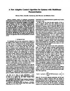
Figure 1 shows a block diagram of the proposed adaptive state filter. In this formulation, there are three neural networks to be constructed, fNN (•), hNN (•), and KNN (•). The networks considered for use are static and dynamic feedforward neural networks 关4,23兴, with well-documented approximation properties 关24兴. Static networks have the structure of FIR-type filters, and training must be performed using all network inputs sampled from the training set, the so-called TF 关4兴. Similarly, dynamic networks have the structure of IIR-type filters, and training must be performed using some network inputs from the training set, whereas others 共delayed outputs兲 using tapped delays 共past predictions兲, the so-called GF 关4,25兴. In training a dynamic network, initially the network predictions are inaccurate and this prevents effective training. In this study, dynamic networks are initially trained using TF, followed by GF 关25兴. 3.2 The Off-Line Training Phase. In the off-line training phase of the filter, in addition to the output measurements used in the training set, ytarget , it is assumed that some reliable state values, xtarget , are also available for use in training. The latter can be obtained from experiments or from the assumed system model, fmod(•) and hmod(•). The former assumption is quite realistic because in a number of real-world systems a limited number of measurements can be collected for variables that might otherwise be very costly to monitor and sense continuously. The effectiveness of the latter assumption about state values depends on the accuracy of the available system model. In some instances, even off-line signal processing methods can be used for extracting state values from input and output measurements. The off-line training is divided into two phases. In the first phase all filter networks are trained as if they were static; that is, they are trained separately using TF. In the second phase the dynamic networks of the filter are coupled and further trained using GF. In the first phase of off-line learning, hNN is developed first, followed by fNN , and then the KNN network. The following objective functions are minimized in this phase of the training process

冦

N P⫺1

E 1⬅

兺

N P⫺1

E 1 共 k⫹1 兲 ⬅

k⫽0 N P⫺1

E 2⬅

兺

k⫽0

N P⫺1

E 3⬅

兺

k⫽0

K

兺 l兺关 yˆ ⫽1

k⫽0

N P⫺1

E 2 共 k⫹1 兲 ⬅

兺 l兺关 xˆ ⫽1

共 k⫹1 兩 k 兲 ⫺y target, l 共 k⫹1 兲兴 2 ,

NN, l

共 k⫹1 兩 k 兲 ⫺x target, l 共 k⫹1 兲兴 2 ,

.

(11)

K

兺 l兺关 xˆ

k⫽0

NN, l

K

k⫽0

N P⫺1

E 3 共 k⫹1 兲 ⬅

Fig. 1 Block diagram of the neural network state filter

⫽1

The error gradients for feedforward networks trained with TF can be obtained by direct application of the chain-rule. The detailed computation of these gradients can be found in many neural networks references, such as 关4,26,27兴. Following completion of the first phase of the off-line learning, GF is used to further train the dynamic networks involved in the state filter, that is the fNN and hNN networks. This form of learning necessitates minimization of a MSP error objective function over a possibly moving window, W s , as follows 关25兴:

NN, l

共 k⫹1 兩 k⫹1 兲 ⫺x target, l 共 k⫹1 兲兴 2 ,

(12)

tandem, by using the response of one network to improve the predictive response of the two others, until all networks produce acceptably accurate MSP responses, as determined by a crossvalidation set. The only measurements used as network inputs in this phase of the off-line training are the delayed system inputs, U(k). All other variables are generated by one of the three networks involved in the state filter. The detailed computation of the error gradients involved in this phase are omitted, but they can be found in a recent publication 关25兴. More recent recurrent learning algorithms can also be considered in this phase of the training that can accelerate the learning process considerably 关28兴.

where the error E(k 0 ,k) depends both on the window location and the prediction point within the window. For off-line learning we select k 0 ⫽1 and W s ⫽N P⫺k 0 . In this phase, the two predictors and the state update network of the filter are further trained in

3.3 The On-Line Training Phase. Neural networks are ‘‘semi-parametric’’ empirical models and therefore they can be ‘‘retrained’’ recursively, on-line training, as new observations become available. This training phase is complicated by the fact that

k 0 ⫹W s

兺

k⫽k 0 ⫹1

k 0 ⫹W s

E 共 k 0 ,k 兲 ⬅

K

兺 l兺共 yˆ l 共 k 兩 k 兲 ⫺y 共 k 兲兲 ,

k⫽k 0 ⫹1

⫽1


0

j

2


the only measurements available are those of the system inputs and outputs, u(k) and y(k), respectively. No state information is available on-line. As in the first phase of the off-line training, during on-line training the networks are decoupled and treated separately. For all the filter networks, only a SSP gradient propagation training is considered because on-line learning with MSP minimization becomes exceedingly complex and impractical. During on-line training, the error function to be minimized is of the form K

E 共 k⫹1 兲 ⬅

兺关 yˆ

l ⫽1

NN, l

共 k⫹1 兩 k 兲 ⫺y target, l 共 k⫹1 兲兴 2 .

(13)

The error gradients used in off-line training must be modified for use in on-line training. For the output predictor network the error gradients can be expressed as

⳵ E 共 k⫹1 兲 ⳵ hNN ⫽2 关 yˆNN 共 k⫹1 兩 k 兲 ⫺ytarget共 k⫹1 兲兴 T . ⳵ whNN ⳵ whNN

冉

冉

⳵ hmod ⫻ ⳵ xˆ共 k⫹1 兩 k 兲 ⫻

冉冊

冊冉

⳵ fmod ⳵ xˆNN 共 k 兩 k 兲

冊冉

冊冊

⳵ KNN ⳵ xˆNN 共 k/k⫺1 兲

⳵ fNN . ⳵ wfNN

(15)

Finally, for the state update network the error gradient can be expressed as

冉

⳵ E 共 k⫹1 兲 ⳵ hNN ⫽2 关 yˆNN 共 k⫹1 兩 k 兲 ⫺ytarget共 k⫹1 兲兴 T ⳵ wKNN ⳵ yˆ共 k⫹1 兩 k 兲

冉

⳵ hmod ⫻ ⳵ xˆ共 k⫹1 兩 k 兲

冊冉

⳵ fmod ⳵ xˆNN 共 k 兩 k 兲

冊冉

冊

⳵ KNN . ⳵ wKNN

冊

(16)

In Eqs. 共15兲 and 共16兲, the contributions of the terms ⑀x (•) and ⑀y (•) to the on-line gradients are ignored. Some of the gradients contained in Eqs. 共14兲 through 共16兲 can be computed using a sensitivity-type network once the specific neural network architecture is selected. The gradients of KNN (•) with respect to wKNN also depend on the specific architecture of the network used, and for a feedforward network they can be obtained using a backpropagation-type procedure. The derivatives of fmod(•) and hmod(•) with respect to the states can be obtained numerically or even analytically, if an analytical form of the assumed model is available. 3.4 Off-Line Versus On-Line Training. It should be noted here that both the off-line and on-line training stages are complementary and essential for training the filter networks. Applying only off-line training will usually not be sufficient. This can be seen by observing Eq. 共8兲, and focusing on the input xˆNN (k ⫹1 兩 k). For the off-line case, xˆNN (k⫹1 兩 k) is given as fmod(xtarget(k),u(k)) and the neural network, KNN(•), essentially attempts to infer the value of xtarget(k⫹1) given the values of xtarget(k) and y(k⫹1). On the other hand, for the on-line case the network KNN(•) attempts to infer xtarget(k⫹1) given y(k⫹1), and the previous estimate xˆNN (k 兩 k), which is not exactly the same as xtarget(k). Therefore, on-line training is more realistic and indeed more accurate than off-line training, allowing the filter to operate in closed-loop form. Filter performance is assessed using the following errors:

⑀act共 k 兲 ⫽

x共 k 兲 ⫺xˆ共 k 兩 k 兲 , x共 k 兲

⑀mod共 k 兲 ⫽

xm 共 k 兲 ⫺xˆ共 k 兩 k 兲 . xm 共 k 兲

4

A Motor-Pump System Case Study

The objective of this case study is to develop an adaptive state filter for simultaneous estimation of a DC motor armature resistance and flux linkage. 4.1 Motor-Pump System Description. The motor-pump system comprises a DC motor, a centrifugal pump, and the associated piping system. The equations governing the operation of the system have been derived by closely following the approaches of 关29,30兴. The armature circuit is expressed as

(14)

For the state predictor network, the equivalent on-line training gradient can be expressed as

⳵ E 共 k⫹1 兲 ⳵ hNN ⫽2 关 yˆNN 共 k⫹1 兩 k 兲 ⫺ytarget共 k⫹1 兲兴 T ⳵ wfNN ⳵ yˆ共 k⫹1 兩 k 兲

The former is a measure of the state estimate accuracy with respect to the ‘‘simulated’’ state value, whereas the latter is a measure of the state estimate accuracy with respect to the state value computed from the assumed model used in off-line training.

(17)


La

dI a 共 t 兲 ⫹R a 共 t 兲 I a 共 t 兲 ⫹K v ⌿ ␻ 共 t 兲 ⫽V a . dt

(18)

The armature resistance is assumed to vary with the armature current, or equivalently with the external load demand, according to R a共 t 兲 ⫽ ␣

dI 2a 共 t 兲 dt

⫹R oa .

(19)

The angular velocity of the combined DC motor and the centrifugal pump is described by

␪mp

d␻共 t 兲 ˙ 共 t 兲 ␻ 共 t 兲 . (20) ⫽⌿I a 共 t 兲 ⫺c m p0 ⫺c m p1 ␻ 共 t 兲 ⫺h 2 M dt

The dynamic equation for the mass flow rate is described by ˙ 共t兲 dM ˙ 2 共 t 兲 ⫺h rr 共 t 兲 M ˙ 2共 t 兲 . ⫽h nn M dt

(21)

The external load on the overall system is varied through variations in h rr (t). The external load cannot be directly measured and therefore it must be estimated. It is assumed that three of the ˙ (t), are measured. motor-pump system states, I a (t), ␻ (t), and M On the other hand, the armature resistance, R a (t), cannot be directly measured and it must be estimated. The set of Eqs. 共18兲 through 共21兲 comprises the motor-pump simulator. Additionally, an assumed motor-pump model is implemented by replacing Eq. 共21兲 with ˙ 共 t 兲 ⫽K mM ␻ 共 t 兲 . M

(22)

Equations 共18兲 through 共20兲 are also used in the assumed motorpump model. However, the physical parameters used in the assumed model are different than those used in the motor-pump simulator. The Tˆ L (t) is estimated from the measured signals, ␻ (t) ˙ (t), using the following semi-empirical relation and M ˙ 共 t 兲␻共 t 兲, Tˆ L 共 t 兲 ⫽kM

(23)

where k⫽0.36 is an empirically determined constant. The Tˆ L (t) is one of the inputs used in the neural state filter. The equations describing the predictor form of the assumed motor-pump model are

冦

m p1 ˆ Iˆ a 共 k⫹1 兩 k 兲 ⫽ f mod ˆ 共 k 兩 k 兲 ,Rˆ a 共 k 兩 k 兲兲 , 共 I a共 k 兩 k 兲 , ␻ m p2 Rˆ a 共 k⫹1 兩 k 兲 ⫽ f mod 共 Iˆ a 共 k 兩 k 兲兲 , m p3 ˆ ␻ˆ 共 k⫹1 兩 k 兲 ⫽ f mod ˆ 共 k 兩 k 兲 ,Tˆ L 共 k 兲兲 , 共 I a共 k 兩 k 兲 , ␻ m p4 6 共 k⫹1 兩 k 兲 ⫽ f mod 共 ␻ M ˆ 共 k 兩 k 兲兲 ,

(24)

m p1 m p2 m p3 m p4 (•), f mod (•), f mod (•), f mod (•) 兴 T where the functions fmod⫽ 关 f mod are the discrete-time equivalents of the assumed motor-pump model. The discrete-time motor-pump model is obtained by applying the standard discretization transformation presented in

SEPTEMBER 2002, Vol. 124 Õ 367

Table 1 Motor-pump system armature resistance and flux linkage filter test set errors

varying number of hidden nodes. The EM networks with the best architecture are determined by trial-and-error to be 8⫺10⫺2 and 10⫺5⫺3, with test errors of E NM SE ⫽3.9% and E NM SE ⫽1.0%, respectively. 4.2.2 State Update Architecture. The state update, KNN (•), is chosen to be a three-layer FMLP static network with 8 nodes in the first layer, corresponding to the inputs, and 2 nodes in the third layer, corresponding to the outputs. The inputs to the first layer are the three measured outputs, the three residuals, and the two corrected state predictions. The two outputs are the two estimated states. The state update network is then trained with the training set and with varying number of hidden nodes. The targets are R ma (k) and ⌿ ma (k), as determined by the assumed motor-pump model. An 8⫺9⫺2 FMLP architecture is determined by trial-anderror to be the best for the state filter update network. The test error for this architecture is E NM SE ⫽0.5%. Fig. 2 Motor-pump system armature resistance and flux linkage filter block diagram

many digital control texts to Eqs. 共18兲 through 共21兲关31兴. In view of the assumed motor measurements hmod⫽ 关 1,0,1,1兴 T . 4.2 Development of the Neural State Filter. To design the neural filter the motor-pump assumed model, fmod and hmod , is used to generate the training set. Zero-mean, white Gaussian process and measurement noise is also added to the simulator such that the measured variables exhibit SNR of 3.0 and 0.5 for low and high noise experiments, respectively. Testing of the filter is performed using the motor-pump simulator, given by Eqs. 共18兲 through 共21兲. In this study, ⌿ is modeled as a slowly varying parameter that is ‘‘constant’’ for a number of transients, and yet acquiring a new value for different set of transients. A training set is constructed consisting of sinusoidal and ramp signals for R a (t), and different constant signals for ⌿. The training set consists of 10,000 samples 共7500 samples for estimation and 2500 samples for the validation or out-of-sample testing used to stop training兲. The test set consists of 2000 samples of sinusoidal and ramp signals with characteristics different than those used in the training set. A block diagram for this filter is depicted in Fig. 2. 4.2.1 Error Model Architectures. The fNN (•) and hNN (•) EM predictors are chosen to be three-layer FMLP dynamic networks with 8 and 10 nodes in the input layer, respectively. The inputs to fNN (•) are the two state predictions from the assumed model, the two predicted state errors, the three measured outputs and the single measured system input. The inputs to hNN (•) are the three output predictions from the assumed model, the three predicted output errors, the three measured outputs and the single measured system input. The number of nodes in the third layer of the predictors is set to two and three, corresponding to the two predicted states and the three predicted system outputs, respectively. The error models are then trained using the training set and 368 Õ Vol. 124, SEPTEMBER 2002

4.3 Development of the Extended Kalman Filter. For comparison purposes, an EKF is designed for estimating the armature resistance and the flux linkage simultaneously. The standard discrete-time formulation of the EKF is used. For a fair comparison with the neural state filters, the previously presented motor-pump predictor and its linearized version, are used in the EKF design. Specifically, in the Prediction Step of the EKF, the predictor equations 共24兲 are used, whereas the same equations are linearized for use in the covariance matrix calculations. In the Update Step of the EKF, the linearized form of the predictor is used in both the update equation of the covariance matrix and the EKF gain matrix calculations. Finally, the noise covariance matrices are calculated using the white Gaussian noise assumptions made in this simulation study. An attempt was also made to develop a linearized KF for the problem at hand. The results were not satisfactory because on a number of simulation studies the linearized filter did not converge. 4.4 Comparison of the Neural Filters and the EKF. The comparison of the neural filters and the EKF for the dual armature resistance and flux linkage study are shown in Table 1, and in Figs. 3 and 4. The simulations presented are for the test set previously discussed. Figures 3 and 4 depict the state estimates as functions of time for the neural filter with and without on-line learning, and for the EKF. All filtering results are compared with the simulated states. The EKF exhibits response similar to the neural filter without on-line learning, while on-line learning improves the state filtering results. In fact, for most of the simulations performed using the neural filter with on-line learning, the mean state estimation error with respect to the simulated states approaches zero. There are some discrepancies in the transients, but the overall responses are comparable, as witnessed by the results of Table 1. This table shows the averages of the state estimation errors with respect to the simulated states and the assumed model states. The most important observation is the value of the average estimation error with respect to the simulated states. Both the neural filter without on-line learning and the EKF show considerable error in Transactions of the ASME

Fig. 3 Motor-pump system armature resistance and flux linkage filter response using the test data set as inputs „high noise environment…

this category because of the uncertainty in the assumed model used in developing them. At the same time, the estimation errors of these two filters with respect to the assumed model are quite low. However, further on-line learning reduces the estimation error with respect to the simulated states, at the expense of the estimation error with respect to the assumed model states. This is expected because the filter with on-line learning drifts away from the assumed model used in the off-line learning. Finally, one should expects that, in general, the estimation results with high

noise to be worse than the corresponding results with low noise. The flux linkage shows an exception to this expectation, but the error difference is very small.

5

The Case Study of a Complex Process System

In this section, an adaptive neural state filter is developed for estimating the UTSG riser void fraction, ␣ R (t).

Fig. 4 Motor-pump system armature resistance and flux linkage filter response using the test data set as inputs „high noise environment…



5.1 Process System Description. A UTSG simulator developed by Choi 关32兴 is adopted for the purpose of this study. Because the open-loop system is unstable, a stabilizing controller is required to allow system operation. The controller structure used with the above UTSG simulator is that proposed by Menon and Parlos 关33兴. The UTSG has one control input, W f w (t), and five disturbance inputs, namely, T hl (t), W pr (t), W st (t), T f w (t), and P pr (t). The only measured output of the UTSG used in this study is L w (t). The UTSG can be represented in the following nonlinear state space representation: dxUTSG共 t 兲 ⫽fUTSG共 xUTSG共 t 兲 ,u UTSG共 t 兲 ,wUTSG共 t 兲兲 , dt

(25)

where the state vector includes both the primary and secondary side states. The system of these nonlinear ordinary differential equations is solved to advance the transient simulation. The measured UTSG output is expressed in terms of its system states, as follows: y UTSG共 t 兲 ⫽L w 共 t 兲 ⫽h UTSG共 xUTSG共 t 兲兲 .

(26)

5.2 Development of the Riser Void Fraction Neural State Filter. The training and test sets used in the development and testing of the neural networks involved in the state filter are a collection of UTSG simulator and assumed model data, corresponding to step and ramp changes in operating power level. Only three of the five disturbances are used, along with the single controlled input of the UTSG. These are collectively referred to by the four-dimensional vector u(k). In addition, the simulator contains white, Gaussian process and measurement noise, such that the measured input and output variables exhibit SNR of 3.0 and 0.5 for low and high noise experiments, respectively. The state filtering method is now applied for estimating the riser void fraction of the UTSG. In this filter, a scheduled 共or piecewise linear兲 UTSG model is used as the filter model, UTSG UTSG f mod (•) and h mod (•), as further described in 关33兴. The training set used in the state filter development comprises of data collected from the scheduled UTSG model subjected to different step and ramp changes in the operating power level. The state values for the riser void fraction are also obtained from the scheduled UTSG model. The test set includes 2 individual tests; a ramp increase of 0.6% per minute from 5% to 10% of full power, and a step increase 15% to 18% of full power. Test sets with both low and high noise, as defined in the previous paragraph, are generated. The neural filter setup used in this case study is shown in Fig. 5. 5.2.1 Error Model Architectures. The f NN (•) and h NN (•) EM predictor networks are chosen to be three-layer FMLP dynamic networks with 7 nodes in the the first layer, and 1 node in the third layer. The inputs to f NN (•) are the state prediction from the assumed model, the predicted state error, the measured output and the four measured system inputs, including the disturbances. The inputs to h NN (•) are the output prediction from the assumed model, the predicted output error, the measured output and the four measured system inputs, including the disturbances. The number of nodes in the third layer of the predictors is set to one, corresponding to the predicted state and the predicted output, respectively. The error models are trained using the training set and a varying number of hidden nodes. The EM networks with the best architecture are determined by trial-and-error to be 7-5-1 and 7-4-1, with test errors of E NM SE ⫽1.98% and E NM SE ⫽1.33%, respectively. 5.2.2 State Update Architecture. The state update, KNN (•), is chosen to be a three-layer FMLP static network with 3 nodes in the first layer, corresponding to the inputs, and 1 nodes in the third layer, corresponding to the outputs. The inputs to the first layer are the measured output, the residual, and the corrected state prediction. The output node is the estimated state. The state update 370 Õ Vol. 124, SEPTEMBER 2002

Fig. 5 Block diagram of the UTSG riser void fraction filter

network is then trained with the training set and with a varying number of hidden nodes. The target in training is the state ␣ mR (k), obtained from the UTSG scheduled model. The best FMLP network is found by trial-and-error to be a 3-4-1 network, with the average test error, E NM SE , computed as 0.11%. 5.3 Development of the Extended Kalman Filter. For comparison purposes, an attempt has been made to develop an EKF for the UTSG case study. The first difficulty in this attempt has been the unavailability of analytical nonlinear or linearized models in state-space form for use in the EKF equations. In particular, the vector functions 共f(•), h(•)兲 and their Jacobians, both used in the EKF algorithm, are related through the differentiation operator, necessitating the availability of an analytic form. Furthermore, the same vector functions 共f(•), h(•)兲 used in the EKF, are assumed to be a perfect representation of the system. In this study, Choi’s simulator 关32兴 is used for testing the effectiveness of all the state filters. As previously described, the simulator is numerically linearized at many steady-state operating points and the resulting linearized models are scheduled 共or fitted兲 to obtain a piecewise linear model 关33兴. The scheduled model is used in the EKF design instead of an analytic nonlinear model. Furthermore, the numerically linearized individual models are used in the EKF error covariance and filter gain calculations. After overcoming these serious modeling difficulties, an EKF is developed for the UTSG riser void fraction. Filter validation is attempted using ramp and step changes in the UTSG operating power level. Process and sensor noise is included in the simulations. The riser void fraction filter did not converge to a steadystate value in any of the simulations performed. Traditionally, EKFs are known to have convergence problems even when analytical nonlinear models of the underlying processes are available. Usually, one would attempt a linearized KF to reduce the impact of convergence problems. In the UTSG case study, a linearized KF did not achieve convergence either. The poor performance of the EKF for the UTSG riser void problem can be attributed to two Transactions of the ASME

Table 2 UTSG process riser void fraction filter test set errors

reasons: 共1兲 the lack of an analytical nonlinear model for use in obtaining a linearized model, and, 共2兲 the introduction of structural modeling differences in the scheduled model used in the EKF design, compared to the simulator used in testing the EKF. 5.4 Comparison of the Neural Filters and the EKF. The comparison of the void fraction neural filters and the EKF are shown in Table 2, and in Figs. 6 and 7. The simulations presented in these figures are for the test set previously discussed. The estimated riser void fraction for the ramp input of the test data set is shown in Fig. 6. The estimated riser void fraction for the step input of the test data set is shown in Fig. 7. These figures depict the state estimates as a function of time for the neural filter with and without on-line learning, and for the EKF. All filtering results are compared with the simulated state. The EKF estimates diverge from the simulated state values, while the neural filter without on-line learning have some steady-state errors. The neural state filtering results obtained in these tests indicate that the riser void fraction filter performs quite well. The filter’s performance is further enhanced by allowing on-line learning. Considering the complexity of the underlying process, the results from both neural filters are quite encouraging. However, on-line learning significantly improves filter performance. Again, for most of the simulations performed using the neural filter with on-line learning the mean state estimation error approaches zero.

There are some discrepancies in the two convergent neural filter transients, but the overall responses are satisfactory, as witnessed by the results of Table 2. This table shows the averages of the state estimation errors with respect to the simulated state and the assumed model state. The most important observation is the value of the average estimation error with respect to the simulated state. The neural filter without on-line learning shows some error in this category because of the uncertainty in the assumed model used in developing it. At the same time, the estimation error of this filter with respect to the assumed model is lower. For the filter with on-line learning the estimation error with respect to the simulated state is further reduced, while also further reducing the estimation error with respect to the assumed model. This is in contrast to the results of the previous case study, though we do not have a reasonable explanation. Finally, one should note that, in general, the estimation results with high noise are worse that the corresponding results with low noise.

6

Summary and Conclusions

A practical algorithm is presented for adaptive state filtering in nonlinear dynamic systems using neural networks. The algorithm involves a prediction step and an update step, similar to the EKF framework. In the proposed formulation an assumed, approximate system model is considered available, though not necessarily in analytic form. Further, an EM is empirically identified to compensate for the unmodeled dynamics. A training procedure is presented for the filter development, consisting of an off-line and an on-line phase. The adaptive state filtering algorithm is used to estimate the armature resistance and the magnetic flux linkage of a motorpump system simultaneously. The armature resistance is considered a system state which cannot be directly measured on-line. This variable has the potential to indicate developing faults in DC motors. During load variations, the magnetic flux linkage is a parameter which varies slowly with time, compared to the armature resistance. Therefore, it is considered as a constant parameter. The resulting neural filter provides quite accurate state estimates. Furthermore, it is observed that the accuracy of the filter is not affected by the high noise environment considered. In all cases

Fig. 6 UTSG process riser void fraction filter response using the ramp input of the test data set „high noise environment…



Fig. 7 UTSG process riser void fraction filter response using the step input of the test data set „high noise environment…

examined, use of the on-line learning has further improved the state filter accuracy. These observations indicate the potential for using such filters in applications involving condition monitoring and fault diagnosis. The second case study presented is that of a UTSG. The UTSG system is open-loop unstable. Thus for the transients considered, a controller is used to stabilize it. An adaptive neural filter is developed to estimate the riser void fraction, a state of the UTSG process system. An EKF is also developed for this parameter. Furthermore, adaptive estimation results with and without on-line learning are presented. The EKF does not converge to a steadystate value. On the contrary the adaptive neural filter converges quite rapidly. Even without on-line learning the neural estimation results are acceptable compared to the EKF, which diverges quite rapidly. However, with the addition of on-line learning there is significant improvement in the neural state estimates, resulting in estimation errors with respect to simulated states of less that 1%. The test results for this adaptive filter affirm that the proposed algorithm can be applied to complex filtering problems with constant or slowly varying parameters. For the two case studies presented it is observed that the accuracy of the filter developed without on-line adaptation is as accurate as the values of the states used in the off-line network training. This fact couples the state estimation accuracy to the accuracy of the assumed system model used in filter design. On-line adaptation further improves the state estimates, though a proper on-line learning algorithm must be used. The on-line learning results further demonstrate that to the extent possible the state estimation error has been decoupled from the accuracy of the assumed model used in the estimators. Finally, our experience indicates that as the uncertainty and complexity of the state filtering problem increase, the benefit of using the proposed algorithm becomes more apparent. It is only then that complex state filters, such as the one proposed in this study, can be justified.

Acknowledgments The authors greatly appreciate the financial support provided to Texas A&M University by the U.S. Department of Energy under grant DE-FG07-89ER12893 and the NASA Johnson Space Center 372 Õ Vol. 124, SEPTEMBER 2002

under grant NAG#9-347. Dr. Atiya would also like to acknowledge the support of NSF’s Engineering Research Center at CalTech.

Nomenclature Acronyms KF, EKF ⫽ Kalman and Extended Kalman Filer UTSG ⫽ U-Tube Steam Generator TF, GF ⫽ Teacher Forcing, Global Feedback SSP, MSP ⫽ Single-step-ahead Prediction, Multi-step-ahead Prediction EM ⫽ ‘‘Error Model’’ FMLP, RMLP ⫽ Feedforward and Recurrent Multilayer Perceptron FIR, IIR ⫽ Finite and Infinite Impulse Response NMSE ⫽ Normalized Mean Squared Error SNR ⫽ Signal-to-Noise Ratio Mathematical Symbols t, k ⫽ continuous time, discrete time x(t), y(t), u(t) ⫽ simulated system state, output and input vector f(•), h(•) ⫽ simulated nonlinear system dynamics z(t), v(t) ⫽ simulated process and sensor noise vectors pˆ(k⫹1 兩 k) ⫽ estimate of a variable p at k ⫹1 using measurements at k fmod(•), hmod(•) ⫽ modeled nonlinear system dynamics xˆ(k⫹1 兩 k), yˆ(k⫹1 兩 k) ⫽ state and output predictions by system model fNN (•), hNN (•) ⫽ neural network state and output EMs Transactions of the ASME

xˆNN (k⫹1 兩 k),yˆNN (k⫹1 兩 k) ⫽ state and output predictions by neural EM xˆNN (k 兩 k) ⫽ adaptive state filter estimate U(k), Y(k) ⫽ vectors containing measured past system inputs and outputs ⑀(k), ⑀x(k⫹1 兩 k), ⑀y(k⫹1 兩 k) ⫽ innovations, and state/output EM errors E(k), Ex(k⫹1 兩 k), Ey(k⫹1 兩 k) ⫽ vectors of past innovations, and past state/output EM errors n y , n u , n e ⫽ number of past output, input and innovations delays n xe , n ye ⫽ number of past EM error delays KNN (•) ⫽ neural network adaptive state filter gain xtarget(k), ytarget(k) ⫽ state and output measurements used in training set E(•), W s , w ⫽ neural network objective function, training window and weights NP, K ⫽ number of training samples l , K ⫽ network output index, number of network outputs ⑀act(k), ⑀mod(k) ⫽ estimation errors relative to simulated and assumed model ⑀act(k), ⑀mod(k) ⫽ average value of estimation errors ⌿, L a , K v ⫽ motor flux linkage, inductance, and motor constant V a (t), I a (t), ␻ (t) ⫽ motor armature voltage, current and angular velocity R a (t), R oa , ␣ ⫽ motor armature resistance 共AR兲, nominal AR, load constant ␪ mp ⫽ motor-pump combined inertia c m p0 , c m p1 ⫽ Motor-pump static and dynamic friction coefficients h 2 , h nn , h rr (t) ⫽ Pump constant, valve/piping flow resistance, pump parameter ˙ (t), Tˆ L (t) ⫽ Pump flow-rate and load M K mM , k ⫽ Empirical pump coefficients in motor-pump model Iˆ a (k 兩 k), Iˆ a (k⫹1 兩 k) ⫽ Motor armature current estimates from assumed model ␻ˆ (k 兩 k), ␻ˆ (k⫹1 兩 k) ⫽ Motor angular velocity estimates from assumed model Rˆ a (k 兩 k), Rˆ a (k⫹1 兩 k) ⫽ Motor armature resistance estimates from assumed model 6 (k⫹1 兩 k) ⫽ Pump flow-rate estimate from M assumed model mp1 mp2 f mod (•), f mod (•), mp3 m p4 (•), f mod (•) ⫽ Discrete-time equivalents of the f mod assumed motor-pump model ˆ m (k) ⫽ Target values of armature resisR m (k), ⌿ tance and flux linkage ˆ NN (k 兩 k) ⫽ Filtered values of armature Rˆ NN,a (k 兩 k), ⌿ resistance and flux linkage W f w (t), T f w (t) ⫽ UTSG feed-water flow-rate and temperature T hl (t) ⫽ UTSG hot-leg temperature W pr (t), W st (t) ⫽ UTSG primary and secondary side flow-rates P pr (t) ⫽ UTSG primary side pressure L w (t) ⫽ UTSG downcomer water level ␣ R (t) ⫽ UTSG void fraction Journal of Dynamic Systems, Measurement, and Control

xUTSG , y UTSG , u UTSG , wUTSG ⫽ UTSG state, output, input and disturbance vectors fUTSG(•), h UTSG(•) ⫽ UTSG simulated nonlinear dynamics UTSG UTSG (•), h mod (•) ⫽ UTSG assumed nonlinear fmod dynamics ␣ m,R (k) ⫽ target value for UTSG void fraction ␣ˆ R (k 兩 k), ␣ˆ R (k⫹1 兩 k) ⫽ UTSG void fraction estimates from assumed model ␣ˆ NN,R (k 兩 k) ⫽ Filtered value of UTSG void fraction

References 关1兴 Kalman, R. E., and Bucy, R. S., 1961, ‘‘New Results in Linear Filtering and Prediction Theory,’’ ASME J. Basic Eng., 83, pp. 95–107. 关2兴 Gelb, A., 1974, Applied Optimal Estimation, MIT Press, Cambridge, MA. 关3兴 Jonsson, G., and Palsson, O. P., 1994, ‘‘An Application of Extended Kalman Filtering to Heat Exchanger Models,’’ ASME J. Dyn. Syst., Meas., Control, 116, pp. 257–264. 关4兴 Haykin, S., 1999, Neural Networks: A Comprehensive Foundation, 2nd Edition, Prentice-Hall, Piscataway, NJ. 关5兴 Lo, J. T-H., 1994, ‘‘Synthetic Approach to Optimal Filtering,’’ IEEE Trans. Neural Netw., 5共5兲 Sept., pp. 803– 811. 关6兴 Elanayar, S., and Shin, Y. C., 1994, ‘‘Radial Basis Function Neural Network for Approximation and Estimation of Nonlinear Stochastic Dynamic Systems,’’ IEEE Trans. Neural Netw., 5共4兲 July, pp. 594 – 603. 关7兴 Annaswamy, A. M., and Yu, S. H., 1996, ‘‘␪-Adaptive Neural Networks: A New Approach to Parameter Estimation,’’ IEEE Trans. Neural Netw., 7共4兲, pp. 594 – 603. 关8兴 Parisini, T., Alessandri, A., Maggiore, M., and Zoppoli, R., 1997, ‘‘On Convergence of Neural Approximate Nonlinear State Estimators,’’ Proceedings of the 1997 American Control Conference, Vol. 3, June, pp. 1819–1822. 关9兴 Alessandri, A., Parisini, T., and Zoppoli, R., 1997, ‘‘Neural Approximators for Nonlinear Finite-Memory State Estimation,’’ Int. J. Control, 67共2兲, pp. 275– 301. 关10兴 Haykin, S., Yee, P., and Derbez, E., 1997, ‘‘Optimum Nonlinear Filtering,’’ IEEE Trans. Neural Netw., 45共11兲 Nov., pp. 2774 –2786. 关11兴 Zhu, R., Chai, T., and Shao, C., 1997, ‘‘Robust Nonlinear Adaptive Observer Design using Dynamic Recurrent Neural Networks,’’ Proceedings of the 1997 American Control Conference, Vol. 2, June, pp. 1096 –1100. 关12兴 Habtom, R., and Litz, L., 1997, ‘‘Estimation of Unmeasured Inputs using Recurrent Neural Networks and the Extended Kalman Filter,’’ International Conference on Neural Networks, Vol. 4, pp. 2067–2071. 关13兴 Dong, X., Qui, L., and Wang, Z., 1997, ‘‘Neural Networks-based Nonlinear Adaptive Filters and On-line Fault Detection,’’ Control and Decision, 12共1兲 Jan., pp. 78 – 87. 关14兴 Lei, J., Guangdong, H., and Jiang, J. P., 1997, ‘‘The State Estimation of the CSTR System Based on a Recurrent Neural Network Trained by HGAs,’’ International Conference on Neural Networks, Vol. 2, pp. 779–782. 关15兴 Schenker, B., and Agarwal, M., 1998, ‘‘Predictive Control of a Bench-Scale Chemical Reactor Based on Neural-Network Models,’’ IEEE Trans. Control Syst. Technol., 6共3兲 May, pp. 388 – 400. 关16兴 Stubberud, S. C., and Owen, M., 1998, ‘‘Targeted On-line Modeling for an Extended Kalman Filter Using Artificial Neural Networks,’’ Proceedings of the 1998 American Control Conference, Vol. 3, June, pp. 1852–1856. 关17兴 Stubberud, S. C., Owen, M., and Lobbia, R. N., 1998, ‘‘Adaptive Extended Kalman Filter Using Artificial Neural Networks,’’ International Journal of Smart Engineering System Design, 1共3兲, pp. 207–221. 关18兴 Durovic, Z., and Kovacevic, B., 1998, ‘‘Adaptive Filtering using Neural Networks Approach,’’ Proceedings of the Mediterranean Electrotechnical Conference, Vol. 1, May, pp. 499–503. 关19兴 Menon, S. K., Parlos, A. G., and Atiya, A. F., 2000, ‘‘Nonlinear State Filtering for Fault Diagnosis and Prognosis in Complex Systems Using Recurrent Neural Networks,’’ 4th Symposium on Fault Detection, Supervision and Safety for Technical Processes, IFAC SAFEPROCESS 2000, June. 关20兴 Parlos, A. G., Menon, S. K., and Atiya, A. F., 1999, ‘‘Adaptive State Estimation Using Dynamic Recurrent Neural Networks,’’ Proceedings of the International Joint Conference on Neural Networks, June. 关21兴 Grewal, M. S., and Andrews, A. P., 1993, Kalman Filtering: Theory and Practice, Prentice-Hall, Upper Saddle River, NJ. 关22兴 Ljung, L., 1999, System Identification: Theory for the User, 2nd Edition, Prentice-Hall, Upper Saddle River, NJ. 关23兴 Narendra, K. S., and Parthasarathy, K., 1990, ‘‘Identification and Control of Dynamic System Using Neural Networks,’’ IEEE Trans. Neural Netw., 1, pp. 4 –27. 关24兴 Barron, A. R., 1994, ‘‘Approximation and Estimation Bounds for Artificial Neural Networks,’’ Journal of Machine Learning, 14, pp. 115–133. 关25兴 Parlos, A. G., Rais, O. T., and Atiya, A. F., 2000, ‘‘Multi-Step-Ahead Prediction in Complex Systems Using Dynamic Recurrent Neural Networks,’’ Neural Networks, 13共4 –5兲, pp. 765–786.


关26兴 Parlos, A. G., Chong, K. T., and Atiya, A., 1994, ‘‘Application of the Recurrent Multilayer Perceptron in Modeling Complex Process Dynamics,’’ IEEE Trans. Neural Netw., 5, pp. 255–266. 关27兴 Williams, R., and Zipser, D., 1989, ‘‘A learning algorithm for continually running fully recurrent neural networks,’’ Neural Comput., 1, pp. 270–280. 关28兴 Atiya, A., and Parlos, A., 2000, ‘‘New Results on Recurrent Network Training: Unifying the Algorithms and Accelerating Convergence,’’ IEEE Trans. Neural Netw., 11, pp. 697–709. 关29兴 Geiger, G., 1984, ‘‘Fault Identification of a Motor-Pump System using Parameter Estimation and Pattern Classification,’’ IFAC 9th Triennial World Congress, Dec.


关30兴 Isermann, R., 1985, ‘‘Process Fault Diagnosis with Parameter Estimation Methods,’’ IFAC Digital Computer Applications to Process Control, Dec., pp. 51– 60. 关31兴 Franklin, G. F., Powell, J. D., and Workman, M., 1998, Digital Control of Dynamic Systems, 3rd Edition, Addison Wesley Longman, Menlo Park, CA. 关32兴 Choi, J. I., 1987, Nonlinear Digital Computer Control for the Steam Generator System in a Pressurized Water Reactor Plant, PhD thesis, MIT, Department of Nuclear Engineering. 关33兴 Menon, S. K., and Parlos, A. G., 1992, ‘‘Gain-Scheduled Nonlinear Control of U-Tube Steam Generator Water Level,’’ Nuclear Science and Engineering, III共3兲, pp. 294 –308.
