An Adaptive UKF Algorithm for the State and ...

Vol. 34, No. 1

ACTA AUTOMATICA SINICA

January, 2008

An Adaptive UKF Algorithm for the State and Parameter Estimations of a Mobile Robot SONG Qi1, 2

HAN Jian-Da1

Abstract For improving the estimation accuracy and the convergence speed of the unscented Kalman filter (UKF), a novel adaptive filter method is proposed. The error between the covariance matrices of innovation measurements and their corresponding estimations/predictions is utilized as the cost function. On the basis of the MIT rule, an adaptive algorithm is designed to update the covariance of the process uncertainties online by minimizing the cost function. The updated covariance is fed back into the normal UKF. Such an adaptive mechanism is intended to compensate the lack of a priori knowledge of the process uncertainty distribution and to improve the performance of UKF for the active state and parameter estimations. The asymptotic properties of this adaptive UKF are discussed. Simulations are conducted using an omni-directional mobile robot, and the results are compared with those obtained by normal UKF to demonstrate its effectiveness and advantage over the previous methods. Key words Adaptive Unscented Kalman filter (UKF), innovation, MIT rule, process covariance

Autonomous control is a key technology for autonomous systems widely used in areas such as satellite clusters, deepspace exploration, air-traffic control, and battlefield management with unmanned systems. Most unmanned systems are highly nonlinear, vary with time, and are coupled; in addition, their operating conditions are dynamic, complex, and unstructured, which represent the unpredictable uncertainties of the control system. The issue of overcoming these uncertainties and achieving high performance control is one of the main concerns in the field of autonomous control. Robust and adaptive control methods followed traditionally suffer from several problems, including conservativeness, online convergence, and the complications involved in their real-time implementation. These problems necessitate the development of a new control algorithm that addresses the situation more directly. To this end, autonomous control methods on the basis of model-reference have become the focus of research, and basic technology and online modeling method has attracted more and more research attention. Neural networks (NN) and NN-based self-learning were proposed as the most effective approaches for the active modeling of an unmanned vehicle in the 1990s[1−2] . However, the problems involved in NN, such as training data selection, online convergence, robustness, reliability, and realtime implementation, limit its application in real systems. In recent years, sequential estimation has become an important approach for online modeling and model-reference control with encouraging achievements[3] . The most popular state estimator for nonlinear system is the extended Kalman filter (EKF)[4] . Although widely used, EKFs have some deficiencies, including the requirement of differentiability of the state dynamics as well as susceptibility to bias and divergence in the state estimates. Unscented Kalman filter (UKF), on the contrary, uses the nonlinear model directly instead of linearizing it[5] . The UKF has the same level of computational complexity as that of EKF, both of which are within the order O(L3 ). Since the nonlinear models are used without linearization, the UKF does not need to calculate Jacobians or Hessians, and can achieve Received November 30, 2006; in revised form April 29, 2007 Supported by National High Technology Research and Development Program of China (863 Program), Hi-Tech Research and Development Program of China (2003AA421020) 1. Robotics Laboratory, Shenyang Institute of Automation, Chinese Academy of Sciences, Shenyang 110016, P. R. China 2. Department of Auto-control, Shenyang Institute of Aeronautical Engineering, Shenyang 110136, P. R. China DOI: 10.3724/SP.J.1004.2008.00072

second-order accuracy, whereas the accuracy of the EKF is of the first order. However, since UKF is with in the framework of the Kalman filter, it can only achieve a good performance under certain assumptions about the system modeling. But in practice, the assumptions are usually not totally satisfied, and the performance of the filter might be seriously downgraded from the theoretical performance or could even diverge. To avoid these problems, an adaptive filter may be applied, which automatically tunes the filter parameter to adapt insufficiently known a priori filter statistics. There have been many investigations in the area of adaptive filter. Maybeck[6] used a maximum-likelihood estimator for designing an adaptive filter that could estimate the system-error covariance matrix. Lee and Alfriend[7] modified the Maybeck0 s methods by introducing a window-scale factor. The new automated adaptive algorithms are integrated into the UKF and can be applied to the nonlinear system. One disadvantage of the algorithm is that it is not very robust numerically. Loebis et al.[8] presented an adaptive EKF method, which adjusts the measurementnoise-covariance matrix, employing the principles of fuzzy logic. However, in practice, it is always difficult to determine the values of the increment of covariance at each sampling time. Mohame et al.[9] investigated the performance of multiple-model-based adaptive Kalman filters for vehicle navigation using GPS. The method assumes a knowledge of all the possible statuses beforehand. In this paper, an on-line innovation-based adaptive scheme of UKF is proposed to adjust the noise covariance. The filter parameter is tuned by using an MIT adaptation rule that minimizes the cost function of the innovation sequence. The asymptotic properties of the proposed adaptive UKF are discussed. Extensive simulations are conducted with respect to the dynamics of an omnidirectional mobile robot. Estimation accuracy is significantly improved with the adaptive approache compared to the conventional UKF.

1

Standard UKF

In this section, the principle of classical UKF is summarized. Consider the general discrete nonlinear system: ( xk+1 = f (x xk , uk ) + w k (1) y k = h (x xk ) + v k

No. 1

SONG Qi and HAN Jian-Da.: An Adaptive UKF Algorithm for the State · · ·

where xk ∈ Rn is the state vector, uk ∈ Rr is the known input vector, y k ∈ Rm is the output vector at time k. w k and v k are, respectively, the disturbance and sensor noise vector, which are assumed to be Gaussian white noise with zero mean. The UKF estimation can be expressed as explained in the following section. Initialization  ¯ 0 = E [x x0 ]  x i h (2)  P0 = E (x x0 − x ¯ 0 )) (x x0 − x ¯ 0 )T Sigma points calculation and time update   χk−1       χ ∗k|k−1         ¯ k|k−1 x          Pk|k−1

h i p ¯ k−1 , x ¯ k−1 ± (n + λ) Pk−1 = x ¡ ¢ = f χ k−1 2n P

wimχ ∗i,k|k−1 ³ ´ ¯ k|k−1 = wic χ ∗i,k|k−1 − x i=0 ³ ´T ¯ k|k−1 · χ ∗i,k|k−1 − x +Q p £ ¤ ¯ k|k−1 , x ¯ k|k−1 ± (n + λ) Pk|k−1 = x ³ ´ = h χ k|k−1 =

i=0 2n P

        χ k|k−1         γ k|k−1      2n P    y¯k|k−1 = wimγ i,k|k−1

(3)

i=0

where  λ  w0m =    n+λ   ¡ ¢  λ  c + n − α2 + β w0 = n+λ   m 1  i = 1, · · · , 2n  w = wic =   i 2 (n  ¡ 2 ¢ + λ)  λ=n α −1 Measurement update  ³ ´ 2n P  c  ¯ P γ − y × = w  ¯ ¯ y y i i,k|k−1 k|k−1 k k   i=0  ³ ´T     γ i,k|k−1 − y¯k|k−1 +R      ³ ´ 2n  P c   ¯ k|k−1 ×   Px¯ky¯k = i=0 wi χ i,k|k−1 − x ³ ´T  ¯ γ − y  i,k|k−1 k|k−1      Kk = Px¯ky¯k Py¯−1  ¯k  ky     Pk = Pk|k−1 − Kk Py¯ky¯k KkT     ³ ´    ¯k = x ¯ k|k−1 + Kk y k − y¯k|k−1 x

2 2.1

(5)

where the variables are defined as follows: {wi } is a set of scalar weights, and n is the state dimension; the parameter ¯ and α determines the spread of the sigma points around x is usually set to 1e − 4 ≤ α ≤ 1. The constant β is used to incorporate part of the prior knowledge of the distribution of x , and for Gaussian distributions, β=2 is optimal. Q and R are the disturbance and sensor-noise covariance, respectively. The linear algebra operation of adding a column to a matrix, i.e., A ±zz , is defined as the addition of the vector to each column of the matrix.

Adaptive UKF Adaptive parameter

There are six parameters in UKF, which are the initial ¯ 0 , initial covariance P0 , process-noise covariance Q, state x measurement-noise covariance R, and unscented transform (UT) parameters α and β. The influence of the initial state and covariance will become asymptotically negligible as more and more data are processed. The values of α and β, which can only affect the higher order of the nonlinear system, have little impact on improving the estimate accuracy of the UKF. As a priori knowledge, the covariance matrices Q and R are most important to the performance and stability of the UKF. If R and/or Q is too small at the beginning of the estimation process, the uncertainty tube around the true value will probably tighten and a biased solution might result if R and/or Q is too large, filter divergence, in the statistical sense, could occur. Additionally, insufficiently known a priori statistics will, in many cases, lead to an inadequate estimation of the weak observable components in the filter. Therefore, in many adaptive filtering algorithms, the covariance matrices R and Q are the main parameters that need to be tuned online. In principle, an adaptive filter can estimate both R and Q. However, adaptive filtering algorithms that try to update both the observational noise and the system noise are not robust, since it is not easy to distinguish between errors in R and Q[10] . The measurement-noise statistics are relatively well known compared to the system-model error. In this study, the adaptive estimation of the processnoise covariance Q is considered. Usually, the process-noise covariance Q is a diagonal matrix. Therefore, the estimation of Q can be simplified as the estimation of its diagonal elements. 2.2

(4)

73

Cost function

An adaptive filter formulation aims to tackle the problem of imperfect a priori information and to achieve a significant improvement in performance over the fixed filter through the filter-learning process based on the innovation sequence. Most innovation-based adaptive filter methods have been developed to minimize the time-averaged innovation covariance. Even though a minimum “true” innovation covariance may be obtained with this criterion, this covariance could be completely different from the one computed by the filter in [11]. Therefore, a recursive algorithm to minimize the difference between the filter-computed and the actual innovation covariance is formulated. The time-averaged innovation covariance is used as an approximation to the actual one: Sk =

1 N

k X

v kv T k

(6)

i=k−N +1

where N is the size of the estimation window. v k is the innovation and can be written as v k = y k − y¯k|k−1

(7)

where y k and y¯k|k−1 are the real measurement (received by the filter) and its estimated (predicted) value, respectively. From the measurement update (5) of the standard UKF, the filter-computed innovation covariance can be obtained as follows:

74

ACTA AUTOMATICA SINICA

Sˆk =

2n X

w ci

³ ´³ ´T γ i,k|k−1 − y¯k|k−1 γ i,k|k−1 − y¯k|k−1 +R

i=0

(8) Then, the criterion function for adaptive UKF is to minimize ·³ ´2 ¸ ¡ 2¢ ˆ (9) Vk = tr ∆Sk = tr Sk − Sk S k is more sensitive to the changes in the system than to ∆S the actual innovation covariance alone[11] . 2.3

Adaptive law

The traditional MIT rule is used in this section to derive the adaptive law. With the MIT rule, the parameters can be adjusted in the negative gradient direction of the criterion function, i.e., q˙km = −η

∂Vk ∂qkm

(10)

where qkm is the m-th diagonal element of the process-noise matrix at time k. η is the tuning rate that determines the convergence speed, which is assumed to satisfy the classic stochastic approximation conditions X X 2 ηk ≥ 0, ηk = ∞, ηk < ∞ (11) k

2.4

k

Adaptive UKF

Equation (10) leads to the following recursive scheme: m qkm = qk−1 −η

∂Vk ·T ∂qkm

(12)

where T is the sampling time or a constant time period. This scheme can be incorporated into the UKF equations to update Q. In order to calculate (11), the derivative of Vk needs to be calculated. From (9), we have µ ¶ ∂ £ ¡ ∂∆Sk2 ∂Vk 2 ¢¤ = tr ∆S = tr = k m ∂qkm ∂qµ ∂qkm ¶ k ∂∆Sk ∂∆Sk tr ∆Sk + ∆Sk ∂qkm ∂qkm

(13)

where ´ ∂∆Sk ∂ ³ ∂Sk ∂ Sˆk = Sk − Sˆk = − m m m m ∂qk ∂qk ∂qk ∂qk

(14)

From (6) and (7), the equation needed for the first term is obtained as follows: ¶ ∂vv T ∂vv k T k v + v = k k ∂qkm ∂qkm i=k−N +1 µ k ´T X y k|k−1 ³ ∂¯ 1 y k − y¯k|k−1 − − m N ∂qk k i=k−N +1 ! ³ ´ ∂¯ yT k|k−1 y k − y¯k|k−1 ∂qkm

∂Sk 1 = ∂qkm N

k X

µ

· ´T 2n ∂¯ y k|k−1 ³ P ∂ Sˆk c = w γ i,k|k−1 − y¯k|k−1 − − i m m ∂qk ∂qk i=0 # (16) ³ ´ ∂¯ yT k|k−1 γ i,k|k−1 − y¯k|k−1 ∂qkm . To implement (14) and (15), ∂¯ y k|k−1 ∂qkm is required. This needs the derivative of the filter equations. For UKF, a recursive algorithm for the gradient of innovation vector can be formulated as follows: Initialization  ∂¯ x0    ∂q m = 0 k    ∂P0 = 0 ∂qkm

(17)

Derivative of sigma points µ √ ¶  χi,k−1 ∂χ ∂¯ x k−1 √ ∂ Pk−1   n + λ i = 1, · · · , n = +  m  ∂qkm ∂qkm  i  ∂qk µ √ ¶ χi,k−1 ∂χ ∂¯ x k−1 √ ∂ Pk−1  = − n + λ    ∂qkm ∂qkm ∂qkm  i−n  i = n + 1, · · · , 2n (18) Derivative propagation  ¯ χ∗i,k|k−1 ∂χ χi,k−1 ∂χ ∂f ¯¯   = ·   m ¯  x x =χχ ∂qk ∂x ∂qkm  i,k−1     2n  X χ∗i,k|k−1 ∂χ ∂¯ x k|k−1  m   w = i   ∂qkm ∂qkm   i=0   ·µ ¶  2n  X χ∗i,k|k−1 ∂χ  ∂Pk|k−1 ∂¯ x k|k−1  c  w = − ×  i  ∂qkm ∂qkm ∂qkm   i=0   ³ ´T ³ ´     ¯ k|k−1 ¯ k|k−1 × χ ∗i,k|k−1 − x + χ ∗i,k|k−1 − x       µ ∗ ¶T #   χi,k|k−1 ∂χ  ∂¯ x k|k−1 ∂Q   − + m ∂qkm ∂qkm ∂qk  à p !    √ χi,k|k−1 ∂χ ∂ P ∂¯ x k|k−1  k|k−1  = + n+λ    ∂qkm ∂qkm ∂qkm   i     i = 1, · · · , n      ! à p    χi,k|k−1 ∂χ ∂ Pk|k−1 ∂¯ x k|k−1 √    = − n+λ   ∂qkm ∂qkm ∂qkm   i−n     i = n + 1, · · · , 2n      ¯   γ i,k|k−1 χi,k|k−1  ∂γ ∂χ ∂h ¯¯   = ·   x ¯x =χχ ∂qkm ∂x ∂qkm i,k|k−1

(19) Gradient of prediction

(15) and the second term can be obtained from (8) as

Vol. 34

2n X γ i,k|k−1 ∂¯ y k|k−1 ∂γ = wim ∂qkm ∂qkm i=0

Derivative updates

(20)

No. 1

                                                                                    

SONG Qi and HAN Jian-Da.: An Adaptive UKF Algorithm for the State · · ·

·µ ¶ 2n X χi,k|k−1 ∂χ ∂¯ x k|k−1 ∂Px¯ky¯k c = w − × i ∂qkm ∂qkm ∂qkm i=0 ³ ´T ³ ´ ¯ k|k−1 × γ i,k|k−1 −¯ y k|k−1 + χ i,k|k−1 − x µ ¶T # γ i,k|k−1 ∂γ ∂¯ y k|k−1 − ∂qkm ∂qkm ·µ ¶ 2n X γ i,k|k−1 ∂γ ∂¯ y k|k−1 ∂Py¯ky¯k c = wi − × ∂qkm ∂qkm ∂qkm i=0 ³ ´T ³ ´ γ i,k|k−1 −¯ y k|k−1 + γ i,k|k−1 − y¯k|k−1 × ¶ # µ γ i,k|k−1 ∂γ ∂¯ y k|k−1 T − ∂qkm ∂qkm −1 ∂Py¯ky¯k ∂Py¯ky¯k −1 = −Py¯−1 P¯ ¯ ¯k ky ∂qkm ∂qkm y ky k ∂Py¯ky¯k −1 ∂Px¯ky¯k −1 ∂Kk = P¯ ¯ − Px¯ky¯k Py¯−1 P¯ ¯ ¯k ky ∂qkm ∂qkm y ky k ∂qkm y ky k µ ¶ ∂Pk|k−1 ∂Px¯ky¯k T ∂Pk ∂Kk T = − Px¯ y¯ − Kk ∂qkm ∂qkm ∂qkm k k ∂qkm ³ ´ ∂¯ y k|k−1 ∂¯ x k|k−1 ∂¯ xk ∂Kk = + y k − y¯k|k−1 − Kk ∂qkm ∂qkm ∂qkm ∂qkm (21)

2.5

q˙ = −¯ g (q)

75

(26)

Because g¯(q) is given by (22), U (q) can be used as a Lyapunov function for the ODE. Therefore, following the results of Ljung in [13], qk will converge to a local minimum of U (q), with a probability 1 as k tends to infinity.

3

Simulation

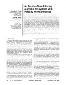
The simulations were carried out with respect to the dynamics of the 3-DOF omni-directional mobile robot developed in the Shenyang Institute of Automation (See Fig. 1).

Asymptotic behavior

In this section, the asymptotic properties of the proposed adaptive UKF are discussed as in [12]. ¯ k is First, assume that the UKF is stable and that x uniformly bounded. Then, from (2)∼(5) and the adap¯ tive UKF ± (17)∼(21), it can be deduced that x k|k−1 and ∂¯ x k|k−1 ∂qkm are stable too. Since η · T is small, the forcing term η · T · ∂Vk /∂qkm in the adaptive UKF algorithm is small too. Consequently, qk ± will change slowly. If the UKF and ∂¯ x k|k−1 ∂qkm are stable, the influence of the ± old parameter estimates on the current xk|k−1 ∂qkm , and consequently, ∂Vk /∂qkm is less gradients ∂x ± relevant. Thus, qk in the UKF equation and ∂¯ x k|k−1 ∂qkm can be approximated to some nominal constant±value q0 . The solutions of the UKF equation and ∂¯ x k|k−1 ∂qkm will be asymptotically close to the steady-state solution (¯ x k|k−1 ± and ∂¯ x k|k−1 ∂qkm ) with qk = q0 . Therefore, the estimate updating equation will approximately coincide with ¯ ∂Vk ¯¯ m qkm = qk−1 −η ·T (22) ∂qkm ¯qk =q0 ± If assuming that the system (¯ x k|k−1 and ∂¯ x k|k−1 ∂qkm ) is stable, its solutions are stationary. Then, in view of the law of large numbers, ∂Vk /∂qkm will approach to g¯m (q0 ) = E(∂Vk /∂qkm ) = ∂U /∂qkm |qk =q0

(23)

£ ¡ ¢¤ U (q0 ) = E(Vk ) = E tr ∆Sk2 (q0 )

(24)

where

Up to some random error, the equation becomes qk = qk−1 − η · g¯(q0 ) · T

(25)

Thus, qk should asymptotically follow the trajectories of the following ordinary differential equation (ODE):

Fig. 1

3.1

3-DOF omni-directional mobile robot

Simulation model

The dynamic model of the mobile robot is[14] :  (2M r2 + 3in Iw )¨ xw + 3i2n Iw y˙ w ϕ˙ w + 3i2n cx˙ w =       in r(β1 u1 + 2u2 cos ϕw + β2 u3 )      2  (2M r + 3in Iw )¨ yw − 3i2n Iw x˙ w ϕ˙ w + 3i2n cy˙ w =  in r(β3 u1 + 2u2 sin ϕw + β4 u3 )       (3in Iw L2 + Iv r2 )ϕ ¨w + 3i2n cL2 ϕ˙ w =      in rL(−u1 − u2 − u3 )

√  β1 = 3 sin ϕw − cos ϕw    √     β2 = 3 sin ϕw − cos ϕw √  β3 = 3 cos ϕw − sin ϕw    √    β4 = 3 cos ϕw − sin ϕw

(27)

(28)

where xw , yw , and φw represent the displacements in x and y directions and the rotation, respectively, u1 , and u3 are the actuated torques on each joint. Other rameters of (27) and (28), and their initial values in simulation are listed in Table 1.

the u2 , pathe

76

ACTA AUTOMATICA SINICA Table 1

3.2

Robot Parameters

Symbols

Physical meanings

Values in simulation

c

Friction coefficient

0.0009 kgm 2 /s

Iw

Inertia on motor axis

M

Mass

120kg

Iv

Inertia

45 kgm2

0.0036 kgm

r

Wheel radius

0.06m

L

Centroid – wheel distance

0.273 m

in

Motor gear ratio

15

2

The state and the measurement vectors are selected as (

*

x = [xw , yw , ϕw , x˙ w , y˙ w , ϕ˙ w ]T

(29)

y = [x˙ w , y˙ w , ϕ˙ w ]T

Assume that the initial state of the system is x T 0 = 0 and the sampling interval is T =0.01 s. The measurements are corrupted by zero © mean-additive ªwhite noise with covariance RT = diag 10−8 , 10−8 , 10−8 . The UKF parameters are  ˆ0 = x T 0 x    ª © −8  −8 −8 −8 −8 −8    Pˆ0 = diag 10 , 10 , 10 , 10 , 10 , 10 R = RT        α = 1 and

β=1

The changes of process noise

The estimation accuracy of the adaptive UKF with respect to the changes of the process-noise statistics is tested. The change of the true process-noise intensity is assumed as  © ª QT 0 = diag 10−12 , 10−12 , 10−12 , 10−8 , 10−8 , 10−8     t < 10 s © −10 ª −10 −10 −6 −6  QT = diag 10 , 10 , 10 , 10 , 10 , 10−6    t ≥ 10 s (30) In UKF, the prior knowledge of the process noise covariance is selected as Q = QT 0 . The velocity-estimation errors of the classical UKF, and the adaptive UKF, under the same condition of the processnoise intensity change, are illustrated in Fig. 2. As can be seen, under incorrect noise information, the classical UKF can not produce optimal estimates due to the violation of the optimality conditions. On the contrary, the estimation errors in the adaptive UKF are quickly overcome and are almost the same as their previous size. 3.3

The changes of the parameters

In this section, the performance of the adaptive UKF for parameter estimations is validated. Here, the UKF is used for the online estimation of both motion states and dynamic parameters of the mobile robot. Such an active estimation is further incorporated into a classical inverse dynamic control (IDC). This is intended to make the robot autonomously adaptive to its internal uncertainties, i.e., to achieve a robust tracking performance

(a) Standard UKF

(b) Adaptive UKF Fig. 2

Vol. 34

State-estimation errors with the time-varying process noise

No. 1

SONG Qi and HAN Jian-Da.: An Adaptive UKF Algorithm for the State · · ·

for the time-varying unknown changes in the vehicle dynamics. The structure of the controller is shown in Fig. 3. The UKF estimations are fed to both the inner and outer loops. For the outer loop, clean states are provided to the classic PD control, whereas for the inner loop, the estimated parameters are provided to the inverse dynamic model enabling it to adaptively track the variations of the actual dynamics.

Fig. 3

Other parameters of the UKF are the same as those mentioned in Section 2. 1. The parameter-estimate results are shown in Fig. 4, from which it can be inferred that the standard UKF with a fixed-value noise covariance cannot track the parameter change due to the lower pseudonoise intensity, which will not provide enough driving power to the parameter estimate. But for the adaptive UKF, the intensity of the pseudonoise will increase during the parameter change by the adaptive parameter update. This can accelerate the convergence of the parameter estimates and make the UKF react quickly and track the abrupt change successfully, after a short period (∼ 3 seconds) of adaptation. Fig. 5 illustrates the performance comparison of the standard UKF and the adaptive UKF with respect to the velocity estimate errors due to the parameter change. The tracking errors of the standard UKF are much more significant than those by the adaptive UKF.

Active model-enhanced IDC

In the following paragraphs, the performance of the adaptive UKF-based and the conventional UKF-based controller are compared. The true values of the friction coefficient and the motor axis inertia are designed to change according to ½ t < 10 s c = c0 , Iw = Iw0 (31) c = c0 + cs , Iw = Iw0 + Iws t ≥ 10 s where the constant change value in 10s is cs =0.0031 kg·m2 /s and Iws =0.0164 kg·m2 . The state vector is subject to zero mean-additive white noise with a covariance: © ª QT = diag 10−14 , 10−14 , 10−14 , 10−10 , 10−10 , 10−10 Other conditions of the system are the same as those in Section 2. 1. So as to estimate the parameters, the joint estimation is used, which treats the parameter vector as a dynamical variable and simply appends it onto the true state vector. Since the dynamics of parameter are unknown, the parameter can be assumed to be a noncorrelated random drift vector and modeled by θk = θk1 + wθk

(32)

where wθk is the Gaussian white noise with zero mean, called the pseudonoise. The pseudonoised is very important for the time-varying parameter estimation[15] . If the pseudonoise is too small, it will not have enough “strength” to drive the UKF to track the parameter change. However, if the pseudonoise is too large, an uncertainty will be introduced, and a biased estimate will be produced. In short, properly adjusting the pseudonoise covariance will improve the convergence rate of the UKF and lead to better tracking of the time-varying parameter. In the simulation, the UKF parameters are designed as  ˆ   cˆ0 = c0 , Iw0 = Iw0   © ª  ˆθ P0 = diag 10−8 , 10−7 © −18 ª  θ   , 10−17   Q = diag 10 Q = QT

77

(a) Standard UKF

78

ACTA AUTOMATICA SINICA

Vol. 34

(b) Adaptive UKF

Fig. 4

Parameter estimation

(b) Adaptive UKF

Fig. 5 ters

4

(a) Standard UKF

State-estimation errors with the time-varying parame-

Conclusion

In this paper, the estimation errors of UKF with unknown noise statistics were analyzed. A novel adaptive UKF was proposed on the basis of the innovation covariance matrix and the MIT adaptive law. In addition, a recursive algorithm has been formulated. Simulations on the dynamics of the omni-directional mobile robot were conducted to verify the proposed scheme. Results show that the adaptive UKF outperforms the conventional UKF in terms of fast convergence and estimation accuracy by tuning the process-noise covariance matrix Q.

No. 1

SONG Qi and HAN Jian-Da.: An Adaptive UKF Algorithm for the State · · · References

1 Pesonen U, Steck J, Rokhsaz K. Adaptive neural network inverse controller for general aviation safety. Journal of Guidance, Control, and Dynamics, 2004, 27(3): 434−443 2 Leitner J, Calise A, Prasad J V R. Analysis of adaptive neural networks for helicopter flight control. Journal of Guidance, Control, and Dynamics, 1997, 20(5): 972−979

79

11 Garcia V J. Determination of noise covariances for extended Kalman filter parameter estimators to account for modeling errors [Ph. D. dissertation], University of Cincinnati, 1997 12 El-Fattah Y M. Recursive self-tuning algorithm for adaptive Kalman filtering. IEE Proceedings, 1983, 130(6): 341−344 13 Ljung L. Analysis of recursive stochastic algorithms. IEEE Transactions on Automatic Control, 1977, 22(4): 551−575

3 Haykin S, deFreitas N. Special issue on sequential state estimation. Proceedings of the IEEE, 2004, 92(3): 399−400

14 Song Y X. Study on trajectory tracking control of mobile robot with orthogonal wheeled assemblies [Ph. D. dissertation], Chinese Academy of Sciences, 2002

4 Lerro D, Bar-Shalom Y. Tracking with debiased consistent converted measurements versus EKF. IEEE Transactions on Aerospace and Electronic Systems, 1993, 29(3): 1015−1022

15 Hill B K, Walker B K. Approximate effect of parameter pseudonoise intensity on rate of covariance for EKF parameter estimators. In: Proceedings of the 30th Conference on Decision and Control. Brighton, England: IEEE, 1991. 1690−1697

5 Julier S J, Uhlmann J K. Unscented filtering and nonlinear estimation. Proceedings of the IEEE, 2004, 92(3): 401−422 6 Maybeck P S. Stochastic Models, Estimation and Control. New York: Academic Press, 1979 7 Lee D J, Alfriend K T. Adaptive sigma point filtering for state and parameter estimation. In: AIAA/AAS Astrodynamics Specialist Conference and Exhibit. Rhode Island: 2004. 1−20 8 Loebis D, Sutton R, Chudley J, Naeem W. Adaptive tuning of a Kalman filter via fuzzy logic for an intelligent AUV navigation system. Control Engineering Practice, 2004, 12(12): 1531−1539 9 Mohamed A H, Schwarz K P. Adaptive Kalman filtering for INS/GPS. Journal of Geodesy, 1999, 73(4): 193−203 10 Blanchet I, Frankignoul C, Cane M. A comparison of adaptive Kalman filters for a tropical Pacific ocean model. Monthly Weather Review, 1997, 125(1): 40−58

SONG Qi Lecturer at the Shenyang Institute of Aeronautical Engineering. She received her Ph. D. degree from the Shenyang Institute of Automation, Chinese Academy of Sciences in 2007. Her research interest covers control techniques for robotic systems, estimation techniques for active model, and fault detection and control. Corresponding author of this paper. E-mail: [email protected] HAN Jian-Da Professor at the Shenyang Institute of Automation, Chinese Academy of Sciences. His research interest covers robust control, estimation techniques for active model, fault detection and control, and on-board path planning for autonomous system. E-mail: [email protected]