Jochen Fro¨hlich*,1 and Kai Schneiderâ ,2 ... proach described in (J. Frö hlich and K. Schneider, Europ. J. Mech. algebra. ...... G. Walter, IEEE Trans. Inform.
JOURNAL OF COMPUTATIONAL PHYSICS ARTICLE NO.
130, 174–190 (1997)
CP965573
An Adaptive Wavelet–Vaguelette Algorithm for the Solution of PDEs Jochen Fro¨hlich*,1 and Kai Schneider†,2 *Konrad–Zuse–Zentrum Berlin, Heilbronner Str. 10, 10711 Berlin, Germany; †Fachbereich Chemie, Technische Chemie, Universita¨t Kaiserslautern, Erwin–Schro¨dinger Straße, 67663 Kaiserslautern, Germany Received December 7, 1995; revised August 20, 1996
The paper first describes a fast algorithm for the discrete orthonormal wavelet transform and its inverse without using the scaling function. This approach permits to compute the decomposition of a function into a lacunary wavelet basis, i.e., a basis constituted of a subset of all basis functions up to a certain scale, without modification. The construction is then extended to operatoradapted biorthogonal wavelets. This is relevant for the solution of certain nonlinear evolutionary PDEs where a priori information about the significant coefficients is available. We pursue the approach described in (J. Fro¨hlich and K. Schneider, Europ. J. Mech. B/Fluids 13, 439, 1994) which is based on the explicit computation of the scalewise contributions of the approximated function to the values at points of hierarchical grids. Here, we present an improved construction employing the cardinal function of the multiresolution. The new method is applied to the Helmholtz equation and illustrated by comparative numerical results. It is then extended for the solution of a nonlinear parabolic PDE with semi-implicit discretization in time and self-adaptive wavelet discretization in space. Results with full adaptivity of the spatial wavelet discretization are presented for a one-dimensional flame front as well as for a two-dimensional problem. Q 1997 Academic Press
1. INTRODUCTION
In recent years the development of multiresolution techniques and wavelets has had a tremendous impact on signal and image processing and many other fields. One of them is the numerical solution of partial differential equations where related ideas have been popular for a long time. Speaking of a PDE we have in mind a partial differential equation with one or more dimensions in space and a time derivative such as typical for conservation laws. Below, the derivative in time is generally discretized by a finite difference scheme while a wavelet discretization is used in space. It is beyond the scope of this introduction to survey all the relevant literature on the application of wavelets to 1
Present address: Institut fu¨r Hydromechanik, Universita¨t Karlsruhe, Kaiserstraße 12, 76128 Karlsruhe, Germany. 2 Present address: Institut fu¨r Chemische Technik, Universita¨t Karlsruhe, Kaiserstraße 12, 76128 Karlsruhe, Germany. 174 0021-9991/97 $25.00 Copyright 1997 by Academic Press All rights of reproduction in any form reserved.
PDEs. A recent attempt has been made by Jawerth and Sweldens [29] to which the reader is referred for more comparative information. The currently existing algorithms can be classified in different ways. First of all, we can distinguish between Galerkin or Petrov–Galerkin schemes, collocation schemes, and algebraic methods. By the latter we mean algorithms which start from a classical discretization, e.g., by finite differences in space. Wavelets are then used in the following stages to speed up the linear algebra. On the other hand, the former two schemes employ wavelets or wavelet-like functions directly for the discretization of the solution and the operators which then induces the subsequent linear algebra. Another classification can be made according to whether a wavelet representation is used for the efficient representation of an operator, the compressed representation of the solution or for both. The first family comprises the ‘‘decomposition schemes.’’ They are based on the fact that wavelets are well localized in physical space and in Fourier space. Hence, an operator which does not too much perturb this localization has, for a given precision, a sparse representation in this basis. It also allows efficient diagonal preconditioning as first observed by Jaffard [28]. Several papers such as [16] have exploited this property of a wavelet basis which can be viewed as a particular multilevel scheme. In [15] a further step has been made incorporating a homogeneous elliptic differential operator into the construction of a biorthogonal basis. Used in a Petrov– Galerkin method it generates a block-diagonal matrix. A remarkable fact when employing wavelets for the discretization of Calderon–Zygmund operators is that both, the operator and its inverse have a sparse representation [37]. The BCR algorithm [6] is an algorithm which can be used to benefit from this fact. Starting from a given matrix it generates a sparse, compressed representation of this matrix which then speeds up linear algebra. When, e.g., resulting from the discretization of a usual difference operator powers of the compressed matrix are even more sparse. This has been used in [21, 1] for linear evolution equations. We subsume the cited methods (and others not mentioned
ADAPTIVE WAVELET–VAGUELETTE ALGORITHM
here for lack of space) as ‘‘decomposition schemes’’ since they start from a regular structure, a uniform discretization or a given matrix, and employ a certain multilevel decomposition which then allows preconditioning or fast algebra. The underlying regular discretization, however, is still present. Although in principle the wavelet multilevel decomposition of the operator could be used in connection with an adaptive decomposition of the solution this is straightforward only for relatively few wavelet methods. Some of these are the ‘‘adaptive evaluation schemes.’’ They are characterized by the fact that the solution is discretized in an adaptive wavelet basis and that a discretized differential operator is applied to the nonuniform unknowns. This typically occurs with explicit time discretization. Examples are [2], the collocation method of [11] based on a particular Sobolev inner product, and the seminal work of Harten [25]. In [26] a broad multiresolution framework is developed which allows to incorporate existing algorithms for hyperbolic conservation laws. The third class of methods are the ‘‘adaptive inversion schemes’’ using simultaneously an adaptive discretization of the unknown and a sparse representation of the operator. Elementary ones such as [34] set up a Galerkin matrix for an adaptive wavelet representation of the solution with the system then to be solved by a standard method. A similar approach is made by [4] using the interpolatory multiresolution of [20] to define an adaptive collocation scheme and to incorporate boundary conditions. The price for the interpolatory basis, however, is that diagonal preconditioning in this basis does not yield bounded condition number [5]. In [49] the authors have developed a similar multilevel collocation method with a linear system to be solved on each level. An early attempt to exploit the compression of the operator and its inverse in a wavelet basis as well as adaptive wavelet representation of the solution has been made in [33] using the theoretical results of [48]. The present work is to be viewed in this line. A different approach has been taken by Perrier and Charton [12] which use an algebraic wavelet method, based on a finite difference scheme, to compress the discrete inverse operator and the actual solution during the time advancement. In all of the three families we find Galerkin, collocation, and algebraic methods or some sort of hybrid approaches. Galerkin schemes potentially allow easier incorporation of the operator into the basis construction, better preconditioning, and are more accessible to theoretical analysis. On the other hand, adaptive transforms and boundary conditions can easier be realized with collocation. The cited collocation schemes, however, generally give up the condition of vanishing moments which may have undesirable consequences. Although starting from different discretization many of the resulting algorithms exhibit similar features. Under certain uniformity conditions Gomes [24]
175
showed that some Galerkin and collocation schemes are equivalent and gives their relation to the method of Harten. When dealing with adaptive discretizations, or boundary conditions, one or the other kind of approach may, however, have conceptual and practical advantages. The present algorithm is an ‘‘adaptive inversion scheme.’’ It employs semi-implicit time discretization for a parabolic PDE and is direct. No linear system needs to be solved due to diagonalizing the stiffness matrix through an appropriate choice of test and trial functions in a Petrov–Galerkin method. The adaptive discretization exploits the compression property of wavelets. In contrast to most signal processing tasks, however, avoiding a costly regular fine grid for the solution of a PDE requires a bottom–up strategy of successive local refinements. Only the subset of the relevant amplitudes is to be computed. This loss of regularity in the index set is an essential difficulty of the approach which we overcome in a particular way in the present paper. Recall that the classical Mallat algorithm can no longer be employed in the lacunary case as it is based on the use of the scaling functions’ coefficients on each scale which do not exhibit the same lacunarity as the wavelet coefficients. In that case it is not clear how to define a suitable projection on the lacunary basis. Let us note that the need of repeated transforms between physical space, i.e., the values at certain grid points and coefficient space, originates in the nonlinearity of the PDE to be solved. For linear operations such as derivation, multiplication by powers of the independent variable etc. the conversion to operations on the wavelet coefficients is possible [31, 21]. For simple nonlinearities the approximate evalution in coefficient space has been studied by Beylkin [7] and others. But for general nonlinear terms such as encountered in combustion modeling the evaluation in physical space seems to be unavoidable. Different strategies to cope with locally refined wavelet basis have been developed. Plantevin [39] constructs an orthonormal basis for a given locally refined dyadic grid. As each modification of the grid requires a new basis construction this can become very costly and seems not to be appropriate for the use in the adaptive discretization of unsteady solutions of PDEs. Ponenti [40] aims at retaining as much of the unmodified compactly supported wavelet basis as possible and succeeds in modifying only those functions that live near the border of the index set of retained wavelets. However, the projection step onto the space spanned by these functions is left unconsidered. Sweldens [46] has developed a strategy which allows almost arbitrary spacing of grid points. A completely irregular discretization, however, makes it difficult to take into account differential operators and to consider smooth bases. The present construction retains the wavelet basis as it is. A lacunary subset is accessed through a simple hierarchical subtraction strategy which permits us to compute individ-
176
¨ HLICH AND SCHNEIDER FRO
ual coefficients of the wavelet series with linear operation count [22]. We give a detailed description of the algorithm for a pure wavelet decomposition and improve the former algorithm by employing the cardinal Lagrange function. This is important as it results in speedup, facilitates the implementation, and allows a clearer analysis of the procedure. Up to here, the approach is similar to the partial collocation method briefly sketched in [35] and the multilevel collocation for frames of [49]. The next important step is to incorporate the differential operator into the basis. Thereby, the related stiffness matrix is diagonalized, avoiding its assembly and inversion. This is particularly favorable when frequently changing the set of active basis functions. We show how the hierarchical decomposition into a lacunary basis of the first part can be adapted to this situation. Thereby, we arrive at an interpolatory transform for a fully adaptive operator–orthogonal wavelet– vaguelette decomposition. It is implemented to solve elliptic problems in one and two space dimensions with periodic boundary conditions. In a final step the algorithm is applied to unsteady reaction–diffusion problems, where the semiimplicit time discretization requires the solution of an elliptic problem in each time step. The set of relevant coefficients to be computed is furnished by a dynamic adaption strategy in coefficient space. The paper is organized as follows. We start in Section 2 with the case of a pure wavelet decomposition and introduce the relevant notation and properties. Furthermore, the inverse transform described here will be retained later on in the complete algorithm. In Section 3 we develop the wavelet–vaguelette decomposition and demonstrate its relation to PDEs. For clearness and ease of notation the method is outlined in these first sections considering the real line. The practical implementation, however, makes use of periodicity. Hence assembling some remarks related to this topic in a separate section seems to be appropriate (Section 4). With the ground prepared in such a way the description of the two-dimensional algorithm in Section 5 can be rather brief. In Section 6 we investigate the essential decay properties of the employed basis function by means of numerical experiments. We finally report sample computations for one- and two-dimensional flames which illustrate the properties of the presented method. 2. RECURSIVE INTERPOLATORY TRANSFORM FOR ORTHOGONAL WAVELETS
The following approach is by no means restricted to orthonormal wavelets but can rather be applied to any basis exhibiting scale separation (even when this only holds in a qualitative way as in [9]). Since orthogonality of the employed basic wavelets is crucial for the later discretization of a PDE we formulate it in these terms right from the beginning.
Assume the set of closed subspaces hVj jj[Z with Vj , Vj11 being a multiresolution analysis (MRA) of L2(R) with scalar product k ., .l and norm i.i2. Let this MRA be generated by some function b(x) through dyadic dilation and translation, i.e., bj,k(x) 5 2j/2b(2jx 2 k)
(2.1)
with hbj,i ji constituting a Riesz basis of Vj, not necessarily being orthogonal. The index convention for other functions below will often be slightly different from (2.1) but made precise each time. Dropping an index means setting it to zero, such as bj 5 bj,0, b 5 b0. The orthonormal scaling function and wavelet function for this MRA are denoted f and c, respectively. The function f can be obtained from b through orthonormalization, but occasionally we also set b 5 f right from the start. Furthermore, we suppose that c has M 1 1 vanishing moments. Due to the MRA structure any function fJ [ VJ can be written as fJ (x) 5
Oc
J,k
fJ,k (x) 5
k
Oc
0,k (x)
1
k
OOd
J2 1
j,k
j50 k
cj,k (x), (2.2)
employing (2.1) for the definition of shift and scale index. Bounds for the translation indices are left unspecified throughout, as these will later be governed by the periodization. The index j 5 0 for the coarsest scale in (2.2) is arbitrary and chosen for later convenience. The filters G nj 5 kfj,n , cj21,0 l, H nj 5 kfj,n , fj21,0 l
(2.3)
are classically used for the transition between both representations in (2.2). They can be obtained in physical space for compactly supported bases and in Fourier space through ˆ *(g) 5 cˆ (2g)/fˆ (g), (2.4) ˆ *(g) 5 fˆ (2g)/fˆ (g), G H where the notation of the Appendix, Eq. (A.5), is employed to emphasize the periodicity of these expressions with respect to g. Given a function f [ L2(R), a projection PJ has to be applied to obtain fJ 5 PJ f. At this point there exists a certain liberty. In [47] different quadrature formulas are developed for this task. The algorithms below rely on the collocation projection as it allows easy connection to values in physical space and successive coarsening of the employed grids. It is defined by fJ
SD SD
k k 5f J . 2J 2
Hence, fJ in (2.2) is determined through
(2.5)
177
ADAPTIVE WAVELET–VAGUELETTE ALGORITHM
fJ (x) 5
O f S2k D S Sx 2 2k D k
J
J
(2.6)
J
Consider the points of nested dyadic grids in R i xj,i 5 j, i, j [ Z 2
with the cardinal Lagrange function SJ of VJ defined by
SJ
SD
H
S DJ
i k 5 di,0, VJ 5 span SJ,k 5 SJ x 2 J 2J 2
verifying the trivial recursion . (2.7)
k
(The scale index for this function is defined without the factor 2 j/2 for ease of notation.) Combining (2.2) and (2.6), the coefficients cJ,k in (2.2) are computed by application of the interpolation filter `
I Jn 5 kSJ,n, fJ,0l, I J* (g) 5 22 J/2 Iˆ *
SD
g , Iˆ *(g) 5 Sˆ(g)/fˆ (g) 2J (2.8)
to the sampled values hf(k/2J)jk. Note that when using wavelets for the discretization of a PDE one would like to exploit the regularity of these functions to obtain efficient approximation of smooth solutions. If, however, the projection step has a truncation error of order much lower than this regularity, it is useless to employ regular wavelets. The classical projection cJ,i 5 f (xJ,i ) to determine fJ in (2.2), for example, converges only like O(h) with h 5 22J. Let us remark that in the L2 setting considered so far interpolation has no meaning. However, as soon as the basis functions have sufficient regularity the same multiresolution can be viewed as a multiresolution in the L2-Sobolev space H r of order r $ 1 without any further change [3]. The existence of a cardinal Lagrange function SJ of VJ is guaranteed by PROPOSITION 1. [50]. For a reproducing kernel Hilbert space V spanned by a Riesz basis hb(x 2 k)jk[Z such that bˆ*(g) ? 0, a cardinal Lagrange function exists and is given by
xj11,2i 5 xj,i , xj11,2i11 5 As xj,i 1 As xj,i11 .
(2.11)
In the following the cardinal interpolation function will play the role of the scaling function employed in the classical algorithm. We therefore define the filters j 5 kSj,m , cj21,0 l Dm
(2.12)
representing collocation projection onto Vj and subsequent projection onto Wj21 when applied to the values h f (xj,i )ji . ` ` Similar to recursions in j for H j , G j one can show PROPOSITION 2. The filters D j in (2.12) verify the recurrence relation `
`
(D j21)*(g) 5 23/2(D j )*(2g), g [ T.
(2.13)
Proof. Equations (2.3), (2.8), (2.12) yield j Dm 5
OG I j l
j l2m .
(2.14)
l
Transfer to Fourier space and application of (2.4) and (2.8) back and forth for j 2 1 and j, respectively, gives the assertion. The following theorem describes the biorthogonality of the filter D J with respect to sampled wavelets and scaling functions. PROPOSITION 3. Given cji , Sji , and D Jn defined by (2.12). Then (i)
OD OD
J n22k
cj,l (xJ,n ) 5 dj,J21 dl,k , j , J,
(2.15)
n
(ii) bˆ(g) , g [ R. Sˆ (g) 5 bˆ*(g)
(2.10)
J n22k Sj,l (xJ,n )
5 0,
j , J,
(2.16)
n
(2.9)
where di,k is the Kronecker symbol. Proof. (i) The sampling theorem in VJ yields
Remark. In [50] the assertion is first proved for b 5 f constituting the kernel of the reproducing kernel Hilbert space V. Equation (2.9) then is deduced as Riesz bases can be converted from one into the other and since S is unique modulo discrete shifts. For spline spaces this equation has already been used by Schoenberg [43].
cj,l (x) 5
O c S2n D S j,l
n
J
J,n (x),
j , J.
(2.17)
Applying scalar products with cJ21,k on both sides and using (2.12), together with the orthogonality of the wavelets proves (2.15).
¨ HLICH AND SCHNEIDER FRO
178 (ii) Analogously, starting from Sj21,k (x) 5
O S S2i D S (x) j21,k
i
J,i
J
(2.18)
with j , J and using the orthogonality of cJ21,i with respect to functions in Vj with j , J, Eq. (2.16) is proved.
ALGORITHM 2. (Inverse wavelet transform).
COROLLARY 1.
On D k
cients in (2.2) is to be computed, it is more economical to use fast convolution by means of FFT employing the technique described in [22]. But this is not the aim here as we consider nonuniform discretization. Similar to the above algorithm we can now devise an inverse transform by successive recombination using the interpolation property of S and the decomposition according to Proposition 3.
j n
5 0, k 5 0, ..., M; j [ Z
(2.19)
n
Proof. Equation (2.19) follows from (2.17) with c (x) replaced by xk. Scalar products with cJ21,k on both sides allow us to use the moment conditions for c. The above shows that, in fact, the filters D j correspond to finite difference formulas of order M 1 1. With the present construction these filters generally do not have compact support which results in most cases from the appearance of the cardinal function. In particular, their decay is algebraic for the multiresolutions of Meyer wavelets employed below and exponential for spline wavelets. The latter also holds for Daubechies wavelets since their cardinal function has noncompact support and decays exponentially [50], except the Haar case which is excluded from here on. Up to now we have used the filter D j only with j 5 J. The following algorithm accomplishes a wavelet transform by successively coarsening the samples. ALGORITHM 1. (Wavelet transform). given samples h f (xJ,i)ji for some J [ N with xJ,i from (2.10). Step 1. fJ (xJ,i ) 5 f (xJ,i ), set j 5 J. Step 2. Compute dj21,k 5
O f (x j
j j,n ) D n22k ,
k5???
(2.20)
n
Step 3. Subtract the contribution from Wj21 at the even grid points fj21(xj21,i ) 5 fj (xj,2i ) 2
Od
j21,k
cj21,k (xj21,i ), i 5 ? ? ? (2.21)
k
iterate Step 2 and Step 3 down to j 5 1. finally compute hc0,iji using hI 0njn from (2.8). The algorithm exploits the fact that if fj is known to belong to Vj, the values at the points xj,i uniquely determine the decomposition in this space by the sampling theorem. These coefficients are computed by the discrete orthogonality relations of Proposition 3. In the periodic case the algorithm even becomes slightly simpler as the final step almost disappears. If, furthermore, the entire set of coeffi-
given coefficients hc0,iji , hdj,i jj50,..., J21,i . Step 1. Set j 5 0 and f0(x0,i ) 5
Oc
0,k
f0,k (x0,i ), i 5 ? ? ?
(2.22)
k
Step 2. Compute fj11 at even grid points fj11 (xj11,2i ) 5 fj (xj,i ) 1
Od
c
j,k j,k (xj,i ),
i 5 ? ? ? (2.23)
k
Step 3. Compute fj11 at odd grid points, fj11 (xj11,2i11 ) 5
O f (x )S 1Od j
j,k
j,k (xj11,2i11 )
(2.24)
k
j,k
cj,k (xj11,2i11 ), i 5 ? ? ?
k
iterate Step 2 and Step 3 for j 5 1, ..., J 2 1. Using (2.7) and (2.11) Steps 2 and 3 can be assembled in fj11(xj11,i ) 5
O f (x j
k
j,k )Sj,k (xj11,i )
1
Od
c
j,k j,k (xj11,i ),
i5???
k
(2.25) which again makes obvious the role of the cardinal function as a substitute for the scaling function. In many applications a priori information can be used for adapting the index set of required coefficients in (2.2) to a given function f. In most cases local importance of fine scale coefficients is due to the presence of singularities or almost-singularities in f. The decay of the wavelet coefficients in scale and space depends on the strength of the singularity and is well known; see [27, 37] and others. Then, the relevant indices for dj,i fulfil a so-called cone condition. It roughly means that at a given point x with finest local scale jx all basis functions on scales j , jx of which the (numerical) support contains x are retained. This property is no prerequisite for the sequel but increases the efficiency of the method. Although generally having noncompact support the filters D j and cj,i exhibit rapid decay and can therefore be truncated in space up to some prescribed tolerance. The operations in step 2 and step 3 of Algorithm 1 then are
179
ADAPTIVE WAVELET–VAGUELETTE ALGORITHM
only carried out on subgrids of hxj,i ji. This increases the savings in each step and requires f to be known only at the union of the involved truncated grids. At the price of a slight error, apart from the one due to the neglect of small coefficients, it yields an O(N) operation count, where N is the number of active basis functions with the order constant depending on the (fixed) length of the employed filters. The operation count for the inverse transform is the same as for Algorithm 1 since the sums in (2.24) are shorter than the one in (2.20). Observe that the error from truncation of the filters does not affect the perfect reconstruction property of the transform and its inverse which is preserved by construction. This was not necessarily the case in [22] where, furthermore, a grid finer than hxj,iji was required for the computation of hdj21,iji to avoid aliasing. As a consequence, the restriction to wavelets well localized in Fourier space such as the Meyer wavelets is removed by the present method. 3. OPERATOR-ADAPTED BASES
An essential step is now the extension of Algorithm 1 to biorthogonal vaguelettes. These can be adapted to certain operators so that such an algorithm may be applied to solve (pseudo-) differential or integral equations by a Petrov–Galerkin scheme. The result is a so-called wavelet– vaguelette decomposition of the solution and the righthand side. Although wavelets are employed to furnish better bases for numerical algorithms than trigonometric polynomials the analysis below relies heavily on the Fourier transform. This technique is well suited for the considered operators and furnishes powerful tools. s Let us denote by s (j )5 om50 am (2fij )m the symbol of a linear operator L of order s [ N0 with constant coeffis cients given by Lu 5 om50 am (x)mu(x). In the following we consider inhomogeneous elliptic differential operators, which means that s (j ) . 0, and we aim to solve the equation Lu 5 f
(3.1)
for u(x). The inverse L21 is represented by the symbol 1/s (j ) and the adjoint L* by the complex conjugate s (j ). The corresponding homogeneous operator which is obtained .by only retaining the highest order term of L is . denoted L with the symbol s 5 as(2fi j ) s. Under suitable conditions (cf. below) one can define the functions
uj,i 5 (L*)21cj,i , ej,i 5 Lcj,i
(3.2)
h j,i 5 (L*) fj,i ,
(3.3)
21
nj,i 5 Lfj,i .
By construction these fulfill the biorthogonality relations
kuj,i , ek,ml 5 dj,k di,m , kh j,i , nj,k l 5 di,k .
(3.4)
Observe that scale invariance (2.1) no longer holds. Apart from a scaling factor depending on s the reason is that an inhomogeneous operator (in contrast to a homogeneous one) involves spatial scales on its own determined by the ratios of different coefficients. These ratios are not altered with j in (3.2) and (3.3). The functions uj,i, ej,i are called vaguelettes [37] as they have similar properties as wavelets (not necessarily being orthogonal) apart from dilation invariance. In particular, they have vanishing moments and fast decay which is shown below. The latter property is of primary concern since it affects the length of the involved filters in the proposed method. We now analyse the functions defined in (3.2) and (3.3), as well as the required operator-adapted cardinal functions. Replacing L with its homogeneous counterpart permits us to verify that for j R y, i.e., for strong . refinement, no degradation occurs. As limjR` (iLcj,i i/iLcj,i i) 5 1 for any suitable norm i.i the homogeneous operator in some sense constitutes a worst-case limit of L when considering its action on elements of Wj with increasing j. Let us start with the following statement which can be deduced from classical Fourier analysis [45]. It determines the decay of a function in physical space by the regularity of its Fourier transform. PROPOSITION 4. Let (dg)kˆf [ L1(R), k 5 0, ..., n,
(3.5)
for some n [ N0. Then xn f [ L`(R). This yields (Riemann-Lebesgue) lim x nf 5 0.
uxuR`
(3.6)
A priori, the Fourier transform in (3.5) has to be understood in a distributional sense. However, in all applications below the considered expressions belong to L2(R) as well (without being mentioned explicitly every time) so that ˆf has the classical L2-meaning. Proposition 4 can now be applied to the functions defined above. PROPOSITION 5. Let L be an inhomogeneous. elliptic operator of order s [ N with symbol s . 0. Let L be the corresponding homogeneous operator containing only the highest order term of L. Consider an MRA with the orthogonal wavelet c fulfilling ud gk cˆ (g)u #
Ck , k 5 0, ..., n; n [ N0, (3.7) (1 1 ugu)r111e
¨ HLICH AND SCHNEIDER FRO
180
for some r $ s, e . 0, and positive constants Ck. Suppose further that
E x c(x) dx 5 0, l
l 5 0, ..., M,
(3.8)
with M $ s. Then the functions u, e, h, n as defined in (3.2) and (3.3) (with u 5 u0,0 etc.) have the same asymptotic decay rate as f and c. This remains true for u, e, n when replacing the inhomogeneous operator by the homogeneous one. Before turning to the proof a few remarks are appropriate. It will become clear that the above assumptions are not necessary conditions for the required decay rates but rather sufficient ones. They are oriented toward the typical MRAs and are well suited for the present examples. For example, an r-regular MRA as defined in [37] is a special case of the considered MRAs and is obtained if (3.5) holds for any n [ N0. The above setting partly results from the desire to cover Meyer wavelets which need not be r-regular. Let us sum up the different parameters characterizing the MRA: r determines the differentiability of f and c, M specifies the number of vanishing moments, and n describes the decay of f, c, and their derivatives up to order r. For particular MRAs these parameters are coupled differently. The Meyer MRA corresponds to infinite r and infinite M while n depends on the construction (n 5 4 in the present computations). Spline wavelets are related to r 5 m 2 1, M 5 m 2 1 and infinite n, where m denotes the (even) order of the spline.
. . the homogeneous operator L with symbol s (0) 5 0 may produce a singularity when dividing by the symbol. As fˆ (0) 5 1, the function h cannot be constructed in a classical . sense. In other words, the equation Lh 5 f cannot .be solved for the right-hand side f. This is different for Le 5 c. In Fourier space (3.8) reads d gl cˆ (g)u g50 5 0, l 5 0, ..., M.
. As M $ s, the expression uˆ 5 cˆ /s still vanishes at g 5 0. Therefore uˆ and its derivatives exist and remain integrable close to the origin also for the homogeneous case. For large g the situation is the same as before. Proposition 5 has been formulated for the scale j 5 0. Due to the rescaling property (2.1) for the functions cj,i it holds for all j. Inequality (3.10) is just modified by supplementary factors 2js or 22js in the constants and rescaling of x by 2j. Other properties can be deduced immediately by similar reasoning. COROLLARY 2. Under the conditions of Proposition 5 it can be shown that c, f [ Hr, e, n [ Hr2s, and u, h [ Hr1s which holds, apart from h, for the homogeneous case as well. Furthermore, u and e have M 1 1 vanishing moments. In the homogeneous case this number modifies to M 1 1 2 s and M 1 1 1 s, respecively. We now turn to the cardinal Lagrange functions in the operator-adapted case and define the spaces
Proof. Equation (3.7) yields d gk cˆ (g) [ L1(R), k 5 0, ..., n.
VL; j 5 spanhLbJ,i ji 5 spanhnJ,i ji .
(3.12)
(3.9) Cardinal functions of these spaces are obtained similarly as before.
Hence from Proposition 4 u c (x)u #
(3.11)
C (1 1 uxu)n
(3.10)
for some positive C. As the wavelet and the orthogonal scaling function are intimately related by construction, (3.7) and, therefore, (3.10) apply for f as well. Obviously, the power r is not required in the above. It serves, however, to prove the same decay for the derivatives in space d xk f and d xk c up to k 5 r, as these are reflected by multiplication with gk in Fourier space. Hence, n and e which are just sums of derivatives up to order s # r decay similarly to . (3.10). This is not modified when replacing L with L. Now consider u defined by uˆ 5 cˆ / s. The existence of the derivatives of cˆ up to k 5 n and s [ C `, s . 0 show that d gkuˆ , k 5 0, ..., n, exist. For small g the symbol tends to a constant while s p gs for large g. Hence, if d gkcˆ [ L1(R) so is d gkuˆ . Application of Proposition 4 shows the decay rate (3.10). The same arguments apply to h. Switching to
PROPOSITION 6. Under the conditions of Proposition 5 the spaces VL; J have a cardinal Lagrange function SL; J if
O s (g 1 2 k)(b )(g 1 2 k) ? 0. J
`
J
j
(3.13)
k[Z
It is given by `
`
SL; J (g) 5
s (g)bJ (g) `
2J ok[Z s (g 1 2Jk)(bJ)(g 1 2Jk)
. (3.14)
. The same remains true for L replaced by L. PROPOSITION 7. Under the conditions of Proposition 5 the functions S, SL, and SL. , if they exist, fulfil the same asymptotic decay estimates (3.10) as f and c. Proof. According to the remark after Proposition 1, Sˆ can be obtained through dividing fˆ by fˆ *, a 1-periodic
181
ADAPTIVE WAVELET–VAGUELETTE ALGORITHM
function. The condition u fˆ *u $ C . 0 has to be fulfilled for S to exist. Hence, uSˆ u # (1/C)u fˆ u. By construction fˆ * has the same number of derivatives as fˆ so that Sˆ fulfills the ` conditions (3.7) and therefore the assertion. SL is obtained analogously as Sˆ replacing fˆ by nˆ . Using Proposition 5 the ` ` above remarks apply identically to SL and SL. . It can be shown that the sets h22sjej,i j, h2sjuj,i j, and h22sjnj,i j form Riesz bases of the spaces they generate [22, 40]. Considering the homogeneous case we have seen that an algorithm involving the functions h j,i would not be practical for large j. Ponenti [40] points out that with increasing j these functions more and more tend to the Greens function of the (inhomogeneous) operator. The common shape for all j destroys the essential zooming-in property. Hence, the functions h2sjh j,i j do not form a Riesz basis in the limit j R y. This important observation triggered the construction in the cited reference where the unknown u in (3.1) is developed in terms of uj,i (and not in terms of cj,i as below). To avoid the use of the unstable set h J,i a modified basis is constructed by means of some finite difference operator compensating the singularity in Fourier space. This makes the construction rather complicated. Furthermore, the projection step depends on this filter and is not obvious. The present algorithm has been developed independently from [40] and is different in the following sense. We do not assume u [ H r1s, as with the representation in terms of uj,i, but rather u [ H r, and we approximate the unknown u in (3.1) by some uJ [ VJ, uJ (x) 5
Oc
0,i
f0,i (x) 1
i
O O d c (x).
J21
j,i
j50
j,i
(3.15)
i
The right-hand side f is then approximated accordingly by fL;J [ VL;J which can be expressed as fL;J (x) 5
O k f, h
n
J,i l J,i (x)
i
5
O k f, h ln (x) 1 O O k f, u l e (x). 0,i
0,i
i
J21
j,i
j50
(3.16)
j,i
i
Inserting (3.15) and (3.16) in (3.1) and applying a Petrov– Galerkin method with test functions hh 0,i , uj,i j shows that, having computed the two rightmost terms of (3.16), the solution uJ is obtained with c0,i 5 k f, h 0,i l, dj,i 5 k f, uj,i l in (3.15). In order to determine these coefficients we use the representation of fL;J in terms of the cardinal Lagrange function SL;J of VL;J analogously to (2.6) fL;J (x) 5
OSD S i
D
i i f J SL;J x 2 J . 2 2
The task then is to accomplish a basis transform from hSL;J,ij to hn0,i, ej,ij when f is given at the required grid points. Due to Proposition 7, the limit j R y does not constitute a problem in the construction. Of course, the sums of f0,i and n0,i in (3.15) and (3.16) can be replaced by linear combinations of S0,i and SL;0,i , respectively. This avoids another type of filters. The biorthogonal basis is now used in the adaptive algorithm of the previous section, replacing SJ,m with SL;J,m and j Dm with j 5 kSL;j,m, uj21,0l. D L;m
This filter fulfills analogous relations as D j apart from scale invariance, in particular discrete orthogonality and vanishing moments. Its decay is determined by Propositions 5 and 7. Another reasoning is illustrative and more direct. It uses the equivalent of Proposition 4 for the Fourier transform fˆ *(g), g [ T (see Appendix). PROPOSITION 8. Under the conditions of Proposition 6 j j has the same decay with m as D m . the filter D L;m Proof. Inserting (3.14) and the definition of uj,i (3.2) into (3.18) leads to cancellation of the symbol s and j 5 D L;m
E
T
`
`
bj,0(g) cj21,0(g) e22fimg `
2J ok[Z s (g 1 2Jk)(bJ )(g12Jk)
dg. (3.19)
The denominator is a smooth nonzero bounded 2f-periodic function which does not alter the decay properties in physical space. In [37] a similar argument is applied to the orthonormalization procedure for the classical wavelets. j The actual computation of D L;m is not based on (3.19) but is described in Section 4. We now obtain the following algorithm for the adaptive solution of (3.1).
ALGORITHM 3. (Operator-adapted decomposition). given index set Ld , LJ 5 h( j, i)u j 5 0, ..., J 2 1, i [ Zj for the amplitudes dj,i of a lacunary wavelet basis in VJ with some J [ N0, a method to evaluate f. Step 0. Compute D Lj , ej21,0 j 5 1, ..., J, where J 2 1 is the finest scale in Ld . Truncate these in space according to a given precision. Step 1. Determine the index set Lx of points xj,i required in the subsequent quadratures. Require the r.h.s. at these points fJ (xj,i) 5 f (xj,i), ( j, i) [ Lx .
(3.17)
(3.18)
Set j 5 J.
(3.20)
¨ HLICH AND SCHNEIDER FRO
182
f˜ˆ (n) 5 ˆf (n), n [ Z
Step 2. dj21,k 5
O
( j,i)[Lx
j fj (xj,i)D L;i 22k , ( j 2 1, k) [ Ld . (3.21)
Step 3. fj21(xj21,i) 5 fj (xj,2i) 2
O
( j21,k)[Ld
dj21,k ej21,k (xj21,i),
(3.22)
( j 2 1, i) [ Lx . iterate Step 2 and step 3 down to j 5 1. final step compute c0,k 5
O f (x 0
0 0,i )I L;k2i
(see Appendix). This generates the periodic analogues g bj,k , g g f j,k , cj,k of the functions bj,k, fj,k, cj,k and the periodic f 5 span hb j MRA of the spaces V j ji i50, ...,2j21 , j [ N0. The index range is due to the periodicity g fj,i 5 fg j,i1k2j (k [ Z) introduced by (4.1). It carries over to all filters and functions in L2(T) below. By construction the orthogonality between shift invariant functions is preserved under (4.1). g Furthermore, f j,k 5 1 for j # 0 as the functions hfj,iji g constitute a partition of unity, and Sg 0,0 5 f0,0 for the same c21,0 for brevity, any reason. Denoting this function by g f ff J [ VJ can then be written as f f (x) 5
(3.23)
In short, the proposed algorithm for the solution of an ODE (3.1) reads as follows: given the values of the r.h.s. at an appropriate set of points, Algorithm 3 is employed to determine the coefficients in the development (3.15) of the solution u. The value of the solution at a point of the grid is then obtained by Algorithm 2. Hence, we employ a vaguelette-decomposition and a wavelet-reconstruction to solve (3.1). This algorithm has been implemented in a periodized version which is discussed in the following section. Observe that when the filters applied in both steps are not truncated and the entire set of basis functions is used, the method is exactly equivalent to a collocation algorithm on the grid hxJ,i ji . The inversion of a linear system is replaced by the application of filters into which the inverse of the operator has been incorporated. As soon as these are truncated this yields a method which is neither a Galerkin nor a collocation method but a hybrid one. It relies on both, the localization in space and frequency, as well as the orthogonality of the wavelets. 4. TRANSITION TO PERIODIC MULTIRESOLUTIONS AND IMPLEMENTATION
The computations below have been executed under periodic conditions. This section therefore gives a comprehensive understanding of what sometimes is just subsumed by the term periodization. We furthermore detail the practical computation of the employed filters. Starting from an MRA on the real line, an MRA on the circle T can be constructed through the projection f˜ (x) 5
O f (x 1 n)
(4.1)
n[Z
from L2(R) onto L2(T) [38, 37]. In Fourier space it reads
O Od
J21 2j21
J
i
j with I L;n 5 kSL;j,n , hj,0l, analogous to (2.8).
(4.2)
j,k
j521 k50
cg j,k (x).
(4.3)
In the periodic setting the indices in scale no longer refer to an affine transform such as (2.1) but rather to applying (2.1) for the nonperiodic counterpart followed by (4.1). A result is that functions and filters are related through recurrence relations in Fourier space [38]. In other words, their Fourier transforms are obtained from the nonperiodic counterparts through coarser and coarser sampling for defj 5 kf f, f fl, n 5 0, ..., 2j 2 creasing j. The values of H j,n j21,0 n 1, for example, can be obtained by `
fj jˆ )k 5 22 H * (H
SD
k , k 5 0, ..., 2j 2 1, 2j
(4.4)
ˆ * from (2.4). Using the mapping (4.1) a cardinal with H Lagrange function is readily obtained similarly to Proposition 1. PROPOSITION 9. Let b fulfil the requirements of Proposif 5 spanhb fj tion 1 and let V J j,i i50, ...,2j21 ( j [ N0) be defined through (2.1), (4.1). Then a cardinal Lagrange function of f exists and is given by V J `
f
Sj (n) 5
`
f b (n) j
, n [ Z. ` f) 2j (b j n
(4.5)
Proof. Since Vj is spanned by shifts of Sj, f Vj is spanned by shifts of ok[Z Sj (x 1 k). Obviously, the interpolation property is preserved through periodization so that this sum indeed is again a cardinal Lagrange function of f Vj and therefore defines f Sj due to its uniqueness. Using (2.9), (4.2), and (A.4) yields (4.5). The nonvanishing denominator is ensured by the condition on b. The required filters in the algorithms devised above have to be determined in a preprocessing step. Throughout, we first compute the exact values and only subsequently truncate the filters with respect to their length. We employ
183
ADAPTIVE WAVELET–VAGUELETTE ALGORITHM
multiresolutions of Battle–Lemarie´ spline wavelets of even order and Meyer wavelets. As both have noncompact support, a few remarks are appropriate. In the present cases the filters H, G, I, D, IL, DL for the nonperiodic MRAs are given explicitly in Fourier space. Recall that these expressions are 1-periodic functions in g (cf. Equation (2.4)). Hence, no error is introduced through the periodization by replacing g with k/2j. This property is not shared by the functions f, c, S, e, etc.; they can be defined in Fourier space but have large or unbounded support in g. Therefore the exact values of these functions have to be deduced from the filters. The values cg J21,0 (xJ,i), for example, are computed by an inverse wavelet transform [38] having initialized with dj,i 5 dj,J21 di,0. In the particular case of Meyer wavelets the compact support in Fourier space can be used to alternatively obtain the function’s values by a DFT of appropriate length since the sum in (A.6) contains at most two entries. As the symbol s does not alter the compact support in frequency space this holds f as well. for u˜ , e˜ , S L For spline wavelets the procedure is more involved. We first compute an interpolation function in the nonperiodic case. Thereto, b 5 Nm with Nm designating the B-spline ` of mth order; hence, Lbj 5 2j/2 LNm(2jx). Relating Nm* to the derivative of the cotangent function [13], for` ` mulae for Lbj* are deduced to express SL;j (g). Analogously to Eq. (2.8) this defines the operator adapted inter` ` ` polation filter I Lj *(g) 5 SL;j (g)/ nj (g). Due to the linearity of the operator L the functions e, n`fulfil ` the same refinement equation as c, f. Hence, j* G L 5 G j*. This is used to compute the function `
`
`
D Lj * (g) 5 G Lj * (g) I Lj * (g)
(4.6)
which is then sampled to accomplish the transfer to the g periodic setting. Subsequently, the values of e j,0 at grid points are generated by the filters as described above. Finally note that different MRAs can, of course, be used to start from. However, we conjecture that a construction in which all the required filters are of compact support cannot be obtained. Daubechies wavelets, for example, have compact support, but the related cardinal function has not [50]. The construction of interpolating orthogonal scaling functions (f 5 S) with compact support is impossible [17]. Such functions can only be obtained by relaxing the requirement of compact support to exponential decay [32, 14]. Another class of interpolatory MRAs with compactly supported functions can be generated by the correlation function of biorthogonal scaling functions [24]. Special cases are the fundamental functions of Lagrange iterative interpolation [19] which is equivalent to the Daubechies autocorrelation function [17] used, e.g., in [20, 5]. Since for these interpolatory MRAs ‘‘wavelets’’ are generally
defined by c(x) 5 f(2x 2 1), fast interpolatory transforms exist, also, in the adaptive case [4]. However, these functions, c, do not have vanishing moments and are nonorthogonal, so that they cannot be used in the present approach. Also the construction of compactly supported operator-adapted wavelets in [15] does not lead to full (bi-)orthogonality of the basis. Further research is required on this topic. 5. TWO-DIMENSIONAL ADAPTIVE ALGORITHM
We now extend the present method to tensor product MRAs defined in [37]. In this framework the solution u is developed as uJ (x, y) 5
OOc kx
ky
0,kx,ky
1
f0,kx,ky (x, y)
OOOOd
J21
3
j50 kx
ky e51
(5.1) e
j,kxky
c ej,kx,ky (x, y)
with
fj,kx,ky (x, y) 5 fj,kx (x) fj,ky ( y)
(5.2)
and
5
cj,kx (x) fj,ky ( y), e 5 1,
c ej,kx,ky (x, y) 5 fj,kx (x) cj,ky ( y), e 5 2, cj,kx (x) cj,ky ( y),
(5.3)
e 5 3.
The method previously described for the solution of an ODE in space can now be applied analogously to the discretization of a PDE in two dimensions. The symbol then depends on two coordinates; i.e., s 5 s (jx , jy). Since it can not generally be decomposed as sx (jx) sy (jy), the resulting operator-adapted cardinal function, vaguelettes, and filters are truely two-dimensional and do not exhibit a structure analogous to (5.2) or (5.3). (An ADI time discretization would yield such an operator at the price of altering finescale components of the solution.) Nevertheless, similar decay in space as proved above can be shown for the twodimensional case using the same techniques. Periodicity is accounted for by the technique of Section 4. 6. NUMERICAL EXPERIMENTS
As a preliminary step the precision of the wavelet transform defined in Section 2 has been investigated for different truncations. Setting f 5 cj,0 ( j 5 21, ..., J 2 1), all coefficients are computed up to J 2 1. The left part of Table I reports the quantity
¨ HLICH AND SCHNEIDER FRO
184
TABLE I Projection Error E1 of Algorithm 1 and E2 of Algorithm 2 for Meyer Wavelets, Cubic Spline Wavelets (m 5 4), and Quintic Spline Wavelets (m 5 6) E1 K
Meyer
Full grid 40 30 20
8.7 2.7 1.6 8.6
E-14 E-5 E-4 E-4
m56 5.7 3.8 4.1 4.5
E-14 E-5 E-4 E-3
E2 m54 3.4 5.6 1.8 5.3
m56
Meyer
E-14 E-7 E-5 E-4
5.5 8.9 9.1 6.3
E-14 E-6 E-5 E-4
7.7 1.4 1.2 1.2
m54
E-14 E-5 E-4 E-3
5.7 2.2 5.7 1.6
E-14 E-7 E-6 E-4
Note. K denotes the number of points from the center of D j, Sj , and cj,i at which summations are stopped, respectively. Finest scale is J 5 10.
E1 5 max hukcj,0, ck,mlQ 2 dj,k d0,m uj,
(6.1)
j,k,m
where the index Q of the scalar product denotes its evaluation by the described recursive quadrature of Algorithm 1. In an analogous way the inverse transform has been tested. The error E2 is defined similarly to (6.1), replacing cj,0 with the function generated by the inverse transform and k? , ?lQ by the exact scalar product. This is realized in starting from dj,0 5 1 for one particular value of j and all other coefficients zero. An inverse transform with truncation and a subsequent exact forward transform without truncation are then executed. A practically relevant example for the presented method is a Helmholtz-type equation arising, e.g., from a semiimplicit time discretization of parabolic equations as applied below. Hence, we set L 5 l 2 xx , l [ R .0;
(6.2)
i.e., s (j) 5 l 1 4f 2j 2, s 5 2. In the sample computations l 5 150 has been used corresponding to the time stepping for the PDE below. Similar to Table I we first consider the influence of the truncation on the orthogonality of the basis functions in the operator-adapted case. Some examples are assembled in Table II. The error E3 is defined as in (6.1) replacing cj,0 by ej,0 and ck,m by uk,m (unfortunately, comparison to a similar table in [22] is not possible for implementational reasons). The level of round-off errors is given by the first line. The precision achieved with truncated filters increases if these have stronger decay, i.e., in case of low regularity of the basis. The observed behavior is related to the filters DL plotted in Fig. 1. According to Proposition 8 their (algebraic) decay is the same as the decay of D which is determined by the properties of the MRA. Indeed, Fig. 1 shows exponential decay when employing spline wavelets and algebraic decay for Meyer wavelets. Next, we report the precision obtained for the solution
of the Helmholtz equation (3.1), (6.2), with a right-hand side such that the exact solution is 2
2
uex 5 e2c (x21/2) , c2 5 16000.
(6.3)
Figure 2 displays the resulting L2-approximation error when computing all wavelet amplitudes of the solution, the L`-error behaves analogously. As stated before, the use of untruncated filters results in a pure collocation method the convergence rate of which is determined by the regularity of the basis functions. With truncated filters the approximation cannot be improved beyond the level induced by the defect in orthogonality. Hence, the error tends to a constant with increasing J when this level is reached. Observe that the values in Fig. 2 nicely correspond to those of Table II (in general a multiplicative factor appears). Furthermore, the result with Meyer wavelets can be compared to Fig. 7 of [22]. A decrease of the error by about two orders of magnitude or, in other terms, half the
TABLE II Projection Error E3 of Algorithm 3 for Meyer Wavelets and Quintic and Cubic Spline Wavelets KD , Ke Full grid 60, 60 40, 40 30, 30 80, 60 40, 30
Meyer 1.5 3.5 3.5 1.6
E-12 E-5 E-4 E-3
1.6 E-5 3.4 E-4
m56 2.8 1.1 8.5 8.9
E-12 E-5 E-4 E-3
7.7 E-7 1.1 E-3
m54 3.5 3.0 2.2 6.1
E-12 E-8 E-5 E-4
2.6 E-9 5.3 E-5
Note. KD , Ke denote the number of points from the center of DL;j and ej,i at which quadrature and summation are stopped, respectively. Finest scale is J 5 10.
ADAPTIVE WAVELET–VAGUELETTE ALGORITHM
185
FIG. 1. Absolute value of the filter D jL;m defined in (3.18) divided by its maximum value versus m for the case of a Meyer MRA, a cubic spline MRA, and a quintic spline MRA with j 5 9 and L from (6.2). For reasons of symmetry only half of the filter is represented.
filter size for the same precision is observed. Due to the interpolatory approach it is also possible now to use spline wavelets in the solution procedure. The results in the right part of Fig. 2 support the above interpretation: for m 5 6 only the stronger truncation influences the accuracy, whereas with m 5 4 the filters could still be shortened without losing considerable precision with respect to the
exact result on the respective grids. To assess the amount of adaptivity which is possible by the approach, Table III displays the number Ne of coefficients which are larger in absolute value than the truncation error e 5 iu 2 uex i2 with the full basis depicted in Fig. 2. Employing only these coefficients in an adaptive computation would lead to drastic savings at the expense of an O(e)-error.
FIG. 2. L2-error iu 2 uex i 2 versus J for the one-dimensional Helmholtz problem solved with Algorithm 3 and different basic multiresolutions. Left: Meyer wavelets. Right: cubic and quintic spline wavelets (all curves of the former are virtually identical).
¨ HLICH AND SCHNEIDER FRO
186 TABLE III
Number of Ne of Significant Amplitudes in the Computations of Fig. 2 (see text) J
7
8
9
10
M full M 80,60 M 40,30
18 18 18
98 98 56
508 146 66
508 146 66
S6 full S6 80,60 S6 40,30
18 18 18
74 74 56
116 116 58
148 148 58
S4 full S4 80,60 S4 40,30
12 12 12
26 26 26
38 38 38
58 58 58
scales. On the other hand, there are bases with low regularity which lead to shorter filters but steeper cones in the index space around singularities or almost-singularities of the solution. Another relation can be drawn to the method of ‘‘approximate approximation’’ proposed by Maz’ya [36]. He considers approximation schemes exhibiting convergence only down to some threshold for the error and, by construction, not below. This exactly corresponds to the saturation observed in this section for truncated filters. 7. ADAPTIVE COMPUTATION OF FLAMES
Similar tests have also been made for a two-dimensional Helmholtz problem with xx in (6.2) replaced by xx 1 yy so that the symbol is s (jx, jy) 5 l 1 4 f 2(j 2x 1 j 2y). The imposed exact solution was (6.3) with (x 2 As)2 replaced by (x 2 As)2 1 ( y 2 As)2. The employed filters have been truncated in the form of a square. Different forms could perhaps slightly improve the efficiency. The results are qualitatively the same as those reported above, so that we restrict ourselves to the case of cubic spline wavelets here. Table IV displays the obtained L2-error for different truncations. The number Ne of amplitudes larger than e 5 iu 2 uex i 2 was 20, 40, 148 for J 5 7, J 5 8, and J 5 9, respectively, except for the shortest filter where we counted 20, 45, and 112. Since, e.g., for J 5 9 uniform discretization yields 262,144 degrees of freedom, this illustrates the increased potential for savings through adaptivity in the two-dimensional case which of course depends on the actual solution. The actual choice of the employed MRA has to depend on the convergence rate in the nontruncated case and the size of the filters which is needed to maintain the required precision. On one hand, there are very regular basis functions and longer filters leading to higher precision on large
The above discretization has been devised for the adaptive solution of a PDE with evaluation of the nonlinear terms in physical space. In this section we report results of one- and two-dimensional computations of this type and detail further features of the algorithm. We consider a reaction–diffusion equation originating from combustion modeling. It describes the propagation of a laminar flame in a quiescent premixed atmosphere and is discussed, e.g., in [10]. For a unitary Lewis number (the ratio of the diffusivity of species to the diffusivity of heat), one-step kinetics, and appropriate initial and boundary conditions the resulting equation for the dimensionless reduced temperature T reads tT 2 =2T 5 r (T ) b2 r (T) 5 (1 2 T ) eb(T21)/(11a(T21)). 2
(7.1)
The variables are scaled such that r unit distance corresponds to the characteristic scale for temperature variations in the flame front. The strong stiffness of this problem results from the fact that this length is typically much smaller than the domain of interest and that, furthermore, the region where r .. 0 is only of size O(b21) in these units. In all computations we employ the semi-implicit time scheme of second order, 3 n11 2 1 n21 2 =2T n11 5 T n 2 1 r (2T n 2 T n21), T T 2Dt Dt 2Dt (7.2)
TABLE IV L2-Error of the Two-Dimensional Helmholtz Problem with Square Truncation of the Fitlers KD , K e Full grid 80, 60 40, 30 30, 20
J57 1.0575 1.0575 1.0575 1.0563
E-3 E-3 E-3 E-3
J58 4.1054 4.1054 4.1054 4.1714
E-4 E-4 E-4 E-4
J59 1.0794 1.0794 1.0796 1.3349
E-4 E-4 E-4 E-4
where the index n represents the time level and Dt the time step. At this occasion we observe that the implicit discretization of the Laplacian is applied for reasons of stability. If, e.g., the second-order term contains a variable coefficient it can be decomposed into a sum of a constant coefficient operator discretized implicitly and a perturbation discretized explicitly in time. This may in some cases yield the required stability. Another solution is to apply
187
ADAPTIVE WAVELET–VAGUELETTE ALGORITHM
FIG. 3. Temperature T 5 T˜ 1 s and reaction rate g (divided by 2.5 for presentation) versus x for a left-traveling thermodiffusive flame front. The dotted curves correspond to t 5 1, the continuous ones to t 5 7. The tics below indicate the centers of the adaptively selected wavelet basis functions computed at the respective times. Their number is larger than the value of Ne mentioned in the text due to the adding of neighbors in scale space. The second cloud for t 5 7 at x 5 0.5 is generated by the periodizing function s(x).
the present algorithm with locally constant coefficients in an iterative scheme as investigated in [30] for uniform discretization. For the one-dimensional computations we consider a steadily propagating flame front similar to the one in [22]. The computational domain [2Lx/2, Lx/2] is mapped onto [0, 1] and a flame is initialized in its middle. For physical reasons the temperature remains constant in a large partition of the domain before and after the front (cf. Fig. 3). The values T 5 0 and T 5 1 are attained with the present scaling. Strictly speaking, these values should be imposed as boundary conditions at y and 2y, but for large Lx they can as well be imposed at x 5 0 and x 5 1, respectively. As long as the front remains sufficiently far from the boundaries it is useful to consider the quantity T˜ 5 T 2 s, where s is a smooth function of x with s(0) 5 0, s(1) 5 1, and all its derivatives vanishing at x 5 0 and x 5 1. Then, T˜ can very well be approximated by a periodic function [18]. (A moving reference frame may be used to generate a steady solution but is avoided here for simplicity.) We employ
S D
s(x) 5 As(1 1 tanh(t tan f 3
f )). 2
(7.3)
from [18] with t 5 5. At each time step the solution is developed in a wavelet sum
T˜ n11(x) 5
O
n11 d j,i cj,i (x).
(7.4)
( j,i)[Ldn11
The index set Ldn11 is determined from T˜n by retaining only those coefficients which are larger than some tolerance e. A moving solution is accounted for by adding to each index ( j, i) of this set its neighboring indices ( j 2 1, i/2), ( j, i 6 1), ( j 1 1, 2i) (if these are not yet present) which then gives Ldn11. The solution is advanced in time by first performing a backward transform of the old solution to the locally refined grid of quadrature points (Algorithm 2). The r.h.s. is then evaluated at these points. Finally, the decomposition into the operator-adapted basis (Algorithm 3) is applied to determine the wavelet amplitudes in (7.4). A result is reported in Fig. 3. This computation for Lx 5 30, a 5 0.8, b 5 10 has been performed with cubic spline wavelets and Dt 5 0.01, J 5 10, e 5 1025. The adaptive discretization follows the front without a problem, requiring a number of significant coefficients of about Ne 5 66, most of the time. Nevertheless, the very sensitive reaction rate is well approximated. With respect to former computations [22] the new projection method leads to reduced cpu time (factor of about 4 for this particular setting) and a reduced number of quadrature points. This is particularly advantageous when the evaluation of the r.h.s. is costly. Let us now solve (7.1) in its two-dimensional form. We
188
¨ HLICH AND SCHNEIDER FRO
FIG. 4. Computation of an elliptic two-dimensional flame front. Left: level lines of the temperature at t 5 1. Right: active coefficients in (5.1) located according to (7.5).
avoid the need for periodization here by considering an outward burning flame which, up to a certain time, can be well approximated with periodic boundary conditions. For small Lewis number and additional radiative heat loss such flames exhibit interesting behavior [42] and have been computed in [8]. The computational domain [2Lx /2, Lx /2]2 is mapped onto [0, 1]2 and at each time step the solution is developed according to (5.1) with a lacunary index set. An analogous sequence of computations as in the onedimensional case is then applied to determine the adaptive wavelet representation of T n11(x, y). For the neighborhood in scale space of each coefficient ( j, ix , iy , e) we consider the points ( j 6 1, ix , iy , e), ( j, ix 6 1, iy 6 1, e), and ( j, ix , iy , mod(e 6 1, 3) 1 1). Figure 4 reports a result obtained by the presented twodimensional adaptive wavelet discretization. We used Lx 5 30, Dt 5 1022, and e 5 1025. The initial state is given by an inclined elliptical flame front which then propagates in an outward direction. Due to the physical stability of thermodiffusive flames at unitary Lewis number [44] the front relaxes to a circle. This example has been selected as its solution and is difficult to resolve, e.g., by parametrized mapping techniques. The left part of Fig. 4 shows level lines of the solution at t 5 1. The right part presents the instantaneous set of adaptively selected coefficients in (5.1). These are represented in the standard way [17, p. 315]; a coefficient d ej,kx,ky is positioned at X 5 2j(1 2 de,2) 1 kx, Y 5 2j(1 2 de,1) 1 ky
(7.5)
with the origin in the upper left corner and the Y-axis directed downwards. As in the one-dimensional case only the selected degrees of freedom are computed while the remaining ones are set to zero. The finest scale in this computation was J 5 7, yielding 128 3 128 possible degrees of freedom. At t 5 1 only 1510, i.e., roughly 10% of them, are required to represent the solution with the desired accuracy. The employed MRA is based on cubic splines. Observe that, although the basis functions reflect to some extent the orthogonal coordinate system, this does not degrade the adaptive discretization in oblique directions. 8. CONCLUSION
The present algorithm is a step towards an atom-like use of wavelet basis functions for the solution of PDEs. We have developed the method in one dimension and have analyzed the resulting filters. The approach has also been extended to a truely two-dimensional fully adaptive wavelet discretization in space. With respect to earlier work [22] the improved methodology results in a clearer presentation, an easier analysis, and increased efficiency. The presented method has been implemented for periodic MRAs and could as well be used for initial value problems in unbounded domains. The direct incorporation of essential boundary conditions is not compatible with the approach since it would destroy the shift invariance of the basis. However, the fictitious domain method reduces the solution of such a boundary value problem to the solution of one or more periodic problems. Hence, employing
189
ADAPTIVE WAVELET–VAGUELETTE ALGORITHM
the proposed adaptive algorithm in this framework will allow us to account for boundary conditions and general domains. See, e.g., [41] for the use with a regular discretization in terms of the scaling function. It is evident that the filters applied in the construction are still unsatisfactory as they do not have compact support right from the start and have to be truncated. The basic multiresolutions with noncompactly supported cardinal functions are not the only reason for this fact. A further difficulty results from the incorporation of the operator inverse which is related to the Greens function. Its advantage is that no linear system needs to be solved. Other approaches in the literature such as [6, 12] start from the representation of the inverse of an operator by means of a wavelet basis (standard or nonstandard form) and determine an approximation by cancelling small matrix entries. This operation is similar to the employed truncation of filters. Hence, the requirement of truncation is no particularity of the present construction but rather a general feature which, nevertheless, would be convenient to overcome. Future research will be concerned with the construction of improved bases for the presented algorithm and its application to the simulation of turbulence [23].
f˜*(g) 5
O f (n)e
, g [ T,
22fig n
n[Z
(A.5)
is obtained from the sampled values of f. It fulfills ˜f*(g) 5
O ˜f (g 1 k),
k[Z
g [ T,
(A.6)
due to the Poisson summation formula. Equations (A.3)– (A.6) remain valid for k [ Z, g [ R, since ˜fˆ k and ˆf* are periodic with period 2j and 1, respectively. ACKNOWLEDGMENT The authors thank F. A. Bornemann for usefull comments during the course of this work.
REFERENCES 1. F. Arandiga and V. F. Candela, and R. Donat, SIAM J. Sci. Comput. 6, 581 (1995). 2. E. Bacry, S. Mallat, and G. Papanicolaou, Math. Mod. Num. Anal. 26, 793 (1992). 3. S. Bertoluzza and G. Naldi, Comp. Appl. Math. 13, 13 (1994). 4. S. Bertoluzza and G. Naldi, preprint, Universita` di Pavia, 1994.
APPENDIX: DEFINITION OF THE EMPLOYED FOURIER TRANSFORMS
The employed Fourier transforms of square integrable functions are
E f (x)e ˜fˆ (n) 5 E ˆf (x)e
ˆf(g) 5
22figx
R
22finx
T
dx, g [ R,
(A.1)
dx, n [ Z,
(A.2)
5. S. Bertoluzza and G. Naldi, Appl. Comp. Harm. Anal. 3, 1 (1996). 6. G. Beylkin, R. Coifman, and V. Rokhlin, Comm. Pure Appl. Math. 44, 141 (1991). 7. G. Beylkin, in Progress in Wavelet Analysis and Applications, Proceedings of the International Conference Wavelets and Applications, Toulouse, 1992, edited by Y. Meyer and S. Roques (Editions Frontiers, Gif-sur-Yvette, 1993), p. 259. 8. H. Bockhorn, J. Fro¨hlich, and K. Schneider. preprint, 1996. 9. R. Brand, W. Freeden, and J. Fro¨hlich, Computing 57, 187 (1996). 10. J. D. Buckmaster and G. S. S Ludford, Theory of Laminar Flames (Cambridge Univer. Press, Cambridge, 1982). 11. W. Cai, and J. Wang, SIAM J. Numer. Anal. 33, 937 (1996).
in the nonperiodic case and the periodic case, respectively. The symbol T designates the circle or one-dimensional torus T 5 R/Z. The brackets around n [ Z in (A.2) are motivated by (4.2). They serve to distinguish (A.2) from the discrete Fourier transform (DFT) of length 2j with some j [ N0 defined by
OSD
(A.3)
O f˜ˆ(k 1 2 z), j
Finally, the transform
14. C. K. Chui and X. Shi, in Mathematical Methods in Computer-Aided Geometric Design, edited by T. Lyche and L. L. Schumaker, (Academic Press, San Diego, 1992), p. 111.
k 5 0, ..., 2j 2 1.
16. W. Dahmen and A. Kunoth. Numer. Math. 63, 315 (1992). 17. I. Daubechies. Ten Lectures on Wavelets (SIAM, Philadelphia, 1992). 18. B. Denet and P. Haldenwang, Combust. Sci. and Tech. 86, 199 (1992).
Considering a 1-periodic function ˜f, the coefficients of a DFT with 2j entries are related to ˜fˆ (n) through the ‘‘aliasing relation’’
z[Z
13. C. K. Chui, An Introduction to Wavelets (Academic Press, Boston, 1992).
15. S. Dahlke and I. Weinreich, Constr. Approx. 9, 237 (1993).
j
2 21 ˜fˆ 5 1 ˜f n e22fink/2j, k 5 0, ..., 2j 2 1. j 2 n50 2j
f˜ˆk 5
12. Ph. Charton and V. Perrier. RAIRO Mode´l. Math. Anal. Numer´. 29, 701 (1995).
19. G. Deslauriers and S. Dubuc, Constr. Approx. 5, 49 (1989). 20. D. L. Donoho, preprint, Stanford University, 1992. 21. B. Engquist, S. Osher, and S. Zhong, SIAM J. Sci. Comput. 15, 755 (1994). 22. J. Fro¨hlich and K. Schneider, Europ. J. Mech., B/Fluids 13, 439 (1994).
(A.4)
23. J. Fro¨hlich and K. Schneider, preprint, University Kaiserslautern, 1995; Appl. Comp. Harm. Anal., to appear. 24. S. Gomes and C. Cuncha, preprint, Universidade de Campinas, Brazil, 1995.
190
¨ HLICH AND SCHNEIDER FRO
25. A. Harten, Comm. Pure Appl. Math. 48, 1305 (1995). 26. A. Harten, SIAM J. Numer. Anal. 33, 1205 (1996). 27. S. Jaffard, C.R. Acad. Sci. Paris I 308, 79 (1989). 28. S. Jaffard, SIAM J. Numer. Anal. 29, 965 (1992). 29. B. Jawerth and W. Sweldens, SIAM Rev., 36, 377 (1994). 30. S. Lazaar, J. Liandrat and Ph. Tchamitchian, C.R. Acad.Sci. Paris I 319, 1101 (1994). 31. P. G. Lemarie´, Rev. Math. Iberoamericana 7, 157 (1991). 32. P. G. Lemarie´-Rieusset and G. Malgouyres. in Wavelets and Applications, edited by Y. Meyer (Masson, Paris, 1992). 33. J. Liandrat and Ph. Tchamitchian, Technical report, ICASE, 1990. 34. Y. Maday, V. Perrier, and J.Ch. Ravel, C.R. Acad.Sci. Paris I 312, 405 (1991).
37. 38. 39. 40. 41. 42. 43. 44. 45. 46.
35. Y. Maday and J.Ch. Ravel, C.R. Acad.Sci. Paris I 315, 85 (1992).
47. 48. 49.
36. V. Maz’ya, in The Mathematics of Finite Elements and Applications. Highlights 1993, edited by J. R. Whiteman (Wiley, New York, 1994).
50.
Y. Meyer, Ondelettes et Ope´rateurs I/II (Hermann, Paris, 1990). V. Perrier and C. Basdevant, Rech. Ae´rosp. 3, 53 (1989). F. Plantevin, Advances in Comp. Math. 4, 293 (1995). P. Ponenti, Ph.D. thesis, University Aix-Marseille I, 1994. Z. Qian and J. Weiss, J. Comput. Phys. 106, 155 (1993). P. Ronney, Combust. Flame 82, 1 (1990). I. J. Schoenberg, J. Approx. Theory 2, 167 (1969). G. I. Sivashinski, Acta Astronaut. 4, 1177 (1977). E. M. Stein and G. Weiss, Fourier Analysis on Euclidian Spaces (Princeton Univer. Press, Princeton, NJ, 1971). W. Sweldens, preprint, IMI, Dept. of Math., Univ. of South Carolina, 1994. W. Sweldens and R. Piessens, SIAM J. Numer. Anal. 31, 1240 (1994). Ph. Tchamitchian, Rev. Mat. Iberoamericana 3, 163 (1987). O. V. Vasilyev, S. Paolucci, and M. Sen, J. Comput. Phys. 120, 33 (1995). G. Walter, IEEE Trans. Inform. Theory 38, 881 (1992).