Aug 10, 1994 - travel via Bangkok, even though it will cost an extra $100. ... database, and in the following section the description of the rules of the system.
An Aditi Implementation of a Flights Database James Harland Kotagiri Ramamohanarao Department of Computer Science Department of Computer Science Royal Melbourne Institute of Technology University of Melbourne GPO Box 2476V, Melbourne, 3001 Parkville 3052 Australia Australia August, 1994
Abstract
We describe the implementation of a ights database in the Aditi deductive database system. Such a database requires a large amount of information to be stored, as well as using a variety of rules to construct ight schedules. Hence we believe that the ights database is a good example of the application of deductive database technology to a realistic problem. The ights database also provides a platform on which new optimisation methods and techniques may be tested and measured, and was the main motivation for the integration of top-down and bottom-up execution mechanisms within Aditi.
1 Introduction A common example application for a deductive database system is a ights database, i.e. a system that can answer questions such as \What is the cheapest ight between Melbourne and New York?". This appears to be a relatively simple problem, as it is merely nding the shortest distance between two nodes in a weighted directed graph. However, in practice there are several implicit constraints and default preferences which complicate the picture; generally, a passenger will usually want a
ight which is as cheap as possible, minimises the time spent in transit, leaves on a speci ed date and arrives before a certain deadline. There also may be circumstances in which the passenger is prepared to accept a seemingly sub-optimal ight in order to satisfy a particular preference. For example, John may ask a travel agent to book him the cheapest ight from Melbourne to London. When told that this will involve a twelve hour wait in transit in Singapore, he then asks that he travel via Bangkok, even though it will cost an extra $100. However, when told that only Shonky Airlines ies to Bangkok, he decides to spend an extra $300 to travel with Deluxe Airways, even though there are two cheaper ights. In this paper we describe our experiences with an implementation of such an application in the Aditi deductive database system, which has been developed at the University of Melbourne [8]. There are several reasons why a ights database seems to be a good choice for a demonstration of deductive database technology. Firstly, recursive rules are needed. In our experience, it seems that deductive databases will not become commercially accepted until they are perceived to be not only at least as reliable, robust and e�cient as relational systems, but also to represent a signi cant advance in technology. As a result, an example implementation, such as the Aditi ights database, will need to incorporate features that relational systems do not have, and recursive rules appears to be the best example 1
of such a feature. In addition, a ight schedule may be simply and elegantly represented by a list of ights, which is generated by building a path through a graph. This requires the use of function symbols, which are absent in most relational systems, and so the path construction must be performed in a host language such as C. The use of both top-down and bottom-up processing, as well as the use of various heuristic methods, also allow an Aditi implementation of a ights database to be signi cantly simpler than a similar system which uses a relational database. Secondly, the recursive rules involved are not those for transitive closure. Such rules can be mimicked by transitive closure operators in languages such as SQL, and often do not appear to be a good use of recursive rules. There has been much work on e�cient algorithms for the computation of transitive closures, and these algorithms can make a deductive database involving transitive closures appear to be an overly complicated solution. Transitive closures, however, are not applicable to this problem; clearly the transitive closure of the basic ights relation is not only massive, it is generally fairly useless. In addition, the problem of nding a ight schedule is not simply a path minimisation problem either. For example, a passenger may not want the cheapest or shortest
ight overall, but the cheapest ight which avoids certain airlines, or minimises the amount of time spent at intermediate stops. Thirdly, large amounts of information are involved. For example, the worldwide timetable for British Airways alone lls a book of around 250 A5 pages. This means that there is no shortage of data for testing purposes or for demonstrating the abilities of the system. For example, we have used the ights database with a base relation containing 54,000 tuples. Whilst this data is realistic, in that it contains the same level of information as in the British Airways timetable, it is ctitious, so that there can be no possible clash with \real" information, and to allow a greater amount of
exibility over the data. Fourthly, there is a variety of constraints associated with queries. For example, a passenger may wish to leave no earlier than 8.00am, unless he can save more than $100 by doing so. In a deductive database system, such constraints can be expressed simply and easily. Finally, the problem is a natural one and easily understood. For these reasons we believe that a ights database is an appropriate demonstration of the abilities of a deductive database system. This paper is organized as follows. In Section 2 we give a brief introduction to the Aditi system and the Nu-Prolog interface to Aditi. In Section 3 we describe the data design for the ights database, and in the following section the description of the rules of the system. In Section 5 we present some performance results for the system, and nally in Section 6 we present our conclusions.
2 Aditi
2.1 The Aditi System
Aditi1 is a deductive database system which has been developed at the University of Melbourne. Programs in Aditi consist of base relations (facts) together with derived relations (rules), and are in fact a subset of (pure) Prolog. Queries are a conjunction of atoms (as in Prolog), and a bottomup evaluation technique is used to answer queries. In nding all answers to a given query, Aditi, like many deductive database systems, uses algorithms and techniques developed for the e�cient answering of queries in relational database systems. Thus we expect that Aditi need not be less e�cient than a relational system for purely relational queries. Aditi also uses several optimisation techniques which are peculiar to deductive databases, particularly for the evaluation of recursive Aditi is named after the goddess in Indian mythology who is \the personi cation of the in nite" and \mother of the gods". 1
2
rules. These techniques include magic sets [1, 4, 3], supplementary magic sets [7], semi-naive evaluation [2], predicate semi-naive evaluation [6], the magic sets interpreter[1], and the context transformation [5]. Aditi is based on a client/server architecture, in which the user interacts with a front-end process, which then communicates with a back-end server process which performs the database operations. There are three kinds of server process in Aditi: the query server, which manages the load that Aditi places on the host machine, database access processes, one per client, which control the evaluation of the client's queries, and relational algebra processes, which carry out relational algebra operations such as joins, selections and projections on behalf of the database access processes. There are four main characteristics of Aditi which, collectively, distinguish it from other deductive databases: it is disk-based, which allows relations to exceed the size of main memory, both for permanent and temporary relations, and includes a bu�er management strategy for managing disk pages; it supports concurrent access by multiple users; it exploits parallelism at several levels; and it allows the storage of terms containing function symbols. It has been possible for researchers to obtain a beta-test version of Aditi since January 1993, and a full release of the system is expected soon. The current version of Aditi comes with a Prolog-like (text-based) interface, a graphical user interface, an interface to the Ingres database system via embedded SQL, and a programming interface to Nu-Prolog. It is also possible to embed top-down computations within Aditi code. For a more detailed description of the Aditi system, the reader is referred to [8].
2.2 The Nu-Prolog Interface
A useful feature of Aditi is that there is a \two-way" interface between Aditi and Nu-Prolog, in that a Nu-Prolog program can make call to Aditi, and an Aditi program can make calls to Nu-Prolog. In this way a Prolog program can be used either as a pre- (or post-) processor for Aditi, or as a tool for intermediate computation within Aditi. This interface is transparent, in that a call to Aditi within a Nu-Prolog program appears just like any other Nu-Prolog call, and a call to Nu-Prolog within an Aditi program looks just like any other Aditi call. This makes it very simple to transfer code between Aditi and Nu-Prolog and vice-versa (provided, of course, that there are no termination problems introduced by the switching of execution mechanism). For example, some Aditi code to nd a list of connections using the Aditi relation paths and then using Nu-Prolog to reverse the list could be written as follows. paths(X, Y, Paths), reverse(Paths, RevPaths)
where reverse is the usual Nu-Prolog reverse predicate. This code would remain the same if the reverse predicate was written in Aditi and the paths predicate was written in Nu-Prolog. In this instance, all the solutions to reverse(Paths, RevPaths) are found, in order to comply with the Aditi computational model. Similarly, a Nu-Prolog program may make a call to an Aditi relation, so that the above goal, with paths being evaluated by Aditi and reverse by Nu-Prolog could be used in a Nu-Prolog program without any change of syntax. In this instance, the Nu-Prolog code may backtrack through the answers to the Aditi goal, if desired. Sometimes a programmer may desire more control than is possible in the transparent interface. For example, it may be useful to make a call to Aditi to determine what ights satisfy a given constraint, and then sort and pretty-print all these ights. For purposes such as this, it is also possible to access Aditi from Nu-Prolog via a table and cursor mechanism. When a call to Aditi is made via the dbQuery predicate, the goal is executed, all the answers to the goal are found, and 3
a handle is returned, which can be used to obtain a cursor, i.e. a pointer to the next tuple in the answer relation. This cursor can then be used to step through the computed answers as many times as required. This not only gives the Nu-Prolog programmer more control over the answers to Aditi queries, but may also improve performance for certain applications, particularly if a given query is asked more than once. The table and cursor mechanism allows the programmer to view the answers in a given order, or to scan the answers more than once, or to sort the answers according to a particular measure. The embedding of Aditi within Nu-Prolog means that we can have a Nu-Prolog program prompt for input, pose the query to the Aditi system, sort the answers according to some user-speci ed preference, and display the ight information for each answer in an interactive and meaningful way. This not only provides more exibility, but also makes it possible to connect existing systems to Aditi in a simple way. The ability to call Nu-Prolog from Aditi means that we can mix top-down and bottom-up computations. For example, in the ights database there is a need to calculate the day of the week corresponding to a given date. The program to compute the day from the date is not particularly large, but contains a signi cant number of tests (such as whether the given year is a leap year or not) and very little data. Whilst this program may be evaluated in either a bottomup or top-down fashion, it turns out that top-down evaluation is signi cantly more e�cient, and hence we make a call to this top-down program from the bottom-up one when the conversion is required. In our experience list processing predicates are also generally signi cantly more e�cient when evaluated top-down than bottom-up. In this way we can make good use of existing e�cient code within the database engine. The ights database has been used as a testbed for Aditi, including evaluation of the performance of the system on a large amount of data, and the performance of various optimization techniques. In the next section we describe the ights system in more detail.
3 Flight Information There are several pieces of information associated with a given ight | its origin and destination, the date and time of departure, the ight number, and so forth. Given that a passenger may wish to travel between two arbitrary places, when it comes to storing this information, it seems natural to store this information for each \hop"; in other words, whilst a given plane may travel from Melbourne to Sydney to Auckland to Honolulu to Los Angeles to Chicago, a passenger may wish to travel from Auckland to Honolulu. Hence we would store this particular sequence as ve separate ights, rather than one long ight. This, of course, is a trade-o�, in that in order to make answering queries faster we increase the storage needed. Given the large amounts of information involved we cannot be too blas�e about storage requirements, but this particular trade-o� seems to be worthwhile. This method of storage also seems to be an appropriate level of granularity, in that a passenger wishing to go to a somewhat obscure place may need to travel to an intermediate hub, and from there to the destination. Storing each \hop" means that such the requisite search can be performed in a more straightforward manner than if each complete plane journey was used as the base unit of information. Another consideration is the patterns involved in airline schedules. Whilst timetables change from time to time, and vary with expected demand from season to season, many schedules are organised on a weekly basis, in that for a speci ed period of time, the schedule is the same from week to week. This means that rather than store each ight individually, which would involve large amounts of repetition, we store the weekly schedule once, and then determine whether there is a
ight on a given date from the appropriate weekly schedule. This, again, is a trade-o�, in that 4
it involves signi cantly less storage, but makes searching for a ight more involved. However, as the extra computation is to determine the day of the week corresponding to a given date, this again seems like a worthwhile compromise, as it would seem that performing this calculation is preferable to storing each ight individually. For these reasons, ight information is stored in a relation flight weekly which has ten attributes, given below: Origin, Destination, Dtime, Atime, Incr, Airline, Number, Day, V from, V to where the ight is from Origin to Destination, departing at Dtime and arriving at Atime. Incr indicates how many days later than departure the ight arrives; this will often be 0, but can also be 1, and sometimes 2. Airline and Number specify the airline and ight number respectively, and Day the day of the week that the ight leaves. V from and V to give the dates between which the schedule is valid. Thus a Qantas ight from Sydney to Los Angeles which departs four times a week during the (southern) winter would be represented as the following four tuples: sydney,los\_angeles,2000,1900,0,qantas,qf007,wed,date(1,6,1994), date(31,8,1994) sydney,los\_angeles,2000,1900,0,qantas,qf007,fri,date(1,6,1994), date(31,8,1994) sydney,los\_angeles,2000,1900,0,qantas,qf007,sat,date(1,6,1994), date(31,8,1994) sydney,los\_angeles,2000,1900,0,qantas,qf007,sun,date(1,6,1994), date(31,8,1994)
Thus to determine whether such a ight departs on the 10th of August 1994, all we need do is determine which day of the week this is. As it is a Wednesday, we nd that there is indeed such a
ight on that day, being Qantas ight 7, departing at 8pm, and arriving in Los Angeles at 7pm on the same day. The way that such a query would be expressed is as follows: ?- day(date(10,8,1994), Day), flight(sydney, los\_angeles, Dtime, Atime, Incr, Airline, Number, Day, V\_from, V\_to), between(V\_from, date(10,8,1994), V\_to).
where day is a relation between dates and days of the week, and between(D1, D2, D3) is true if D2 is a date no earlier than D1 and no later than D3. In the system we incorporate such queries into the flight between relation. Another way to store this information is to use one tuple to represent the four ights by combining the \day" argument into a list of days on which the ight leaves. Thus the above four tuples would become sydney,los\_angeles,2000,1900,0,qantas,qf007,[wed,fri,sat,sun], date(1,6,1994),date(31,8,1994)
Whilst this involves a desirable saving in space, this requires indexes which involve set membership, as we clearly wish to be able to use the \day" argument as an index. Such indexing is not yet possible in Aditi, and so we use the four tuple version. 5
Clearly this is not the only way that the ight information can be organized. For example, another possibility is to store in a base relation each \expected" link, rather than all links, together with a list of the intermediate stops. Thus a ight from Sydney to Los Angeles that travels via Auckland and Honolulu may be stored with Sydney and Los Angeles stored as separate attributes, together with the list [Auckland, Honolulu]. This means that a ight from Sydney to Los Angeles can be discovered directly from the base relation. The trade-o� this time is that all possible \sub ights" between Sydney and Los Angeles must be stored, such as Auckland to Los Angeles, and Sydney to Honolulu. This clearly involves a larger amount of storage space than the scheme in which each hop is stored. Storing each hop is also simpler and more exible, as it allows ights to be put together in arbitrary ways, rather than in xed patterns, and the alternative scheme would still require similar facilities for putting together a trip from the basic ight information. Perhaps most importantly, storing each expected ight path makes the design appear to be unnecessarily complicated, which is of paramount concern in a demonstration system. Another point that should be made is that individual airlines may store their data in individual formats, and so putting together a ight schedule may require converting between schemas and formats. The Aditi system, which has interfaces to other database systems such as Ingres as well as its own storage format, provides a uniform framework for combining such information. All ight data could be accessed via the Aditi system, in which would reside the rules for putting a schedule together. This may not be the most e�cient method from a performance point of view, but it simpli es the design, and may in fact be the only feasible way to combine data in di�erent formats.
4 Assembling a Flight Schedule Retrieving ight information is one thing; putting together a schedule is quite another | not only do we need to satisfy constraints such as allowing a minimum time between ights (as well as any constraints given by the passenger), but due to the large amounts of information involved, we also need to ensure that the search procedure is feasible. This is particularly acute when there is no direct ight from the origin to the destination, as the choice of intermediate stops is, in principle, vast, but in practice there are usually only a few realistic choices. For example, if a passenger wishes to travel from Melbourne to Los Angeles, we need only consider trans-Paci c ights, and there is no need to consider ights to Europe or Asia. Hence the search procedure should avoid consideration of ights via London, Bombay or Tokyo, but presumably consider ights via Sydney, Auckland or Honolulu. Various heuristics may be employed to determine the most suitable routes, such as the locating the nearest city with a direct ight to the destination, travelling to the nearest \hub" airport, or nding the route which is shortest in time and/or distance. Given that such heuristics will vary according to local airline policies and may change with time, we have chosen to use a single relation to guide the search, which allows us maximum exibility. This relation speci es which intermediate stops are feasible for a given origin and destination. Clearly this method allows
exibility, in that if there are some exceptions to a general rule, then the exceptions can be explicitly listed in the relation, with the general rules being used to implicitly de ne the less problematic cases. The intention of the feasible relation is to exclude from consideration routes which are clearly of no bene t. In the above example, the feasible relation includes the tuples melbourne, auckland, los_angeles melbourne, sydney, los_angeles melbourne, honolulu, los_angeles
6
but London, Bombay and Tokyo are not included as feasible intermediate stops for a trip between Melbourne and Los Angeles. This relation is de ned using both a base relation and a set of rules. Clearly it is possible to de ne this relation by a base relation alone, but this is somewhat wasteful. In addition, there are certain regularities in the feasible routes which rules can express succinctly, such as commutativity. For example, it is feasible to travel from Melbourne to Auckland to Honolulu to Los Angeles, and hence it is feasible to travel in the reverse direction as well. In addition, it is simple to state principles such as \Honolulu is a feasible stop for all ights from Melbourne to somewhere in North America" as rules. Such a rule is given below. feasible(melbourne, honolulu, Z) :- place(Z, north_america).
It is possible to extend this scheme, of course. A useful extension would be to introduce a second relation, a subrelation of the feasible relation, which would be a more precise heuristic, in that whilst there may be many feasible routes, there is often a smaller number of choices which make the most sense. In the above example, whilst it is feasible to travel from Melbourne to Los Angeles via Honolulu or Auckland, it is usually simpler to travel via Sydney, from which there are direct ights to Los Angeles, and so this latter choice would be the recommended route, chosen from amongst the feasible ones. Thus when searching for an intermediate stop between Melbourne and Los Angeles (assuming that there are no direct ights), the search procedure would rst consider Sydney as the intermediate stop, and only if there are no suitable ights via Sydney would it consider Auckland or Honolulu. If the latter choices fail, then the search procedure would report that there is no feasible
ight. In this case the passenger may wish to ask a more general query, considering somewhat more bizarre routes such as travelling via Tokyo, Bangkok or London. However, in order to keep things simple, we have only used the feasible relation in this system. Thus the default code to nd a ight schedule is as follows: trip(From, To, Ddate, Earliest, Latest, Stime, Ddate1, Dtime, Adate, Atime, [flight(From, To, Ddate1, Dtime, Adate, Atime, A, N)]) :flight_between(From, To, Ddate, Earliest, Latest, Ddate1, Dtime, Adate, Atime, A, N). trip(From, To, Ddate, Earliest, Latest, Stime, Ddate2, Dtime, Adate1, Atime1, [flight(Stop,To,Ddate1,Dtime1,Adate1,Atime1,A,N)|F]) :feasible(From, Stop, To), trip(From, Stop, Ddate, Earliest, Latest, Stime, Ddate2, Dtime, Adate, Atime, F), NewEarliest = Atime + 100, NewLatest = Atime + Stime, flight_between(Stop, To, Adate, NewEarliest, NewLatest, Ddate1, Dtime1, Adate1, Atime1, A, N).
Note that trip is similar to the transitive closure of the ight between relation, but it is actually subtlely di�erent, due to the restriction that each \hop" must be feasible. The rst ve arguments 7
to ight between must be bound, specifying the desired origin, destination, departure date, and the earliest and latest times of departure. The other arguments return the actual ight information, including departure and arrival times, the airline and ight number, and the number of \hops" used in the trip. Note also that the arrival date is given as well, as for some ights such as international
ights, this may be di�erent from the departure date. In fact, the departure date is given as well, as the actual day that the ight leaves could be later than the date speci ed. Currently the system only searches within a departure \window" of 48 hours or less; longer periods will not result in any more ights being found. It is possible to extend this to be any interval, so that searches such as that for a ight any time in the next four days might be simply expressed. The rst six arguments to trip must be bound, not only to include the information passed to
ight between, but also to include the maximum amount of time the customer is prepared to wait in transit. Once the recursive call to trip has returned, the window is then shifted, so that there is at least one hour between ights. This form of the rules is almost left-linear, in that the recursive call to the trip predicate comes before the call to ight between. This means that the algorithm for nding ights may be thought of as nding a feasible intermediate place from which a direct ight can be found, and then nding a way to get to the intermediate place. This is due to the recursive call to trip occurring before the call to flight between, and as the default strategy in Aditi is to evaluate goals left-to-right, the recursive call is evaluated rst. As a result, the ight paths conclude with the longest possible hop, in that direct ights from intermediate stops are preferred over indirect ones. In particular, the algorithm does not search for an indirect ight from an intermediate place when a direct ight exists. This seems to be a reasonable choice, in that the passenger presumably wants to get to his or her destination with as little interruption as possible. However, there are clearly some ight paths which are excluded this way. To include such paths, the trip relation can be rewritten so that the recursive call to the trip relation comes after that for the ight between relation, which corresponds to nding a feasible intermediate stop from which one can continue the trip. This clearly includes all of the previous cases, as well as some in which an indirect route is used instead of a direct one. For this reason we have chosen to use the \left-linear" form of the rules. In addition, rules of this form are generally more e�cient than the corresponding right-linear ones, as transformations such as magic sets tend to result in simpler code for the left-linear case, and to minimise the number of tuples in the magic set. This introduces another problem, in that to use the left-linear form of the rules and to collect the ight path requires some list processing. For example, a right-linear version of (a simpli ed form of) the trip relation which collects the ight path may be given as follows: trip(From, To, [From, To]) :- flight(From, To). trip(From, To, From.Path) :- flight(From, Stop), trip(Stop, To, Path).
However, the left-linear version cannot collect this path in the correct order without some list processing. trip(From, To, [From, To]) :- flight(From, To). trip(From, To, NewPath) :- trip(From, Stop, Path), flight(Stop, To), append(Path, [To], NewPath).
8
One way to minimise the amount of list processing is to collect the list in reverse order, and then reverse the list. trip(From, To, Path) :- trip1(From, To, Rev), reverse(Rev, Path). trip1(From, To, [To, From]) :- flight(From, To). trip1(From, To, To.Path) :- trip1(From, Stop, Path), flight(Stop, To).
This feature was one of the key motivations for allowing Aditi relations to make calls to NuProlog, as list processing predicates such as append and reverse are generally much faster when evaluated top-down than when evaluated bottom-up. This adaptability of the key rules in the system allowed us to experiment with various kinds of rules quickly and easily. It seems that an important feature of a deductive database approach to this problem is that the rules of the database are fairly short and simple, making it relatively straightforward to alter the way in which the schedule is generated, if desired. As this is basically a problem involving heuristic search, being able to change the way the search is done is an important consideration. Another heuristic which seems useful is to use the same airline for the duration of the trip. This will often reduce the cost, as well as simplify travel arrangements. Also, the passenger may wish to specify a particular airline, due to a personal preference or some inducement such as a frequent
yer discount. The way that this is expressed in the system is to add an extra argument to the trip relation, so that the recursive rule becomes trip_air(From, To, Ddate, Earliest, Latest, Stime, Airline, Ddate2, Dtime, Adate1, Atime1, [flight(Stop,To,Ddate1,Dtime1,Adate1,Atime1,Airline,N)|F]) :feasible(From, Stop, To), trip_air(From, Stop, Ddate, Earliest, Latest, Stime, Airline, Ddate2, Dtime, Adate, Atime, F), NewEarliest = Atime + 100, NewLatest = Atime + Stime, flight_between(Stop, To, Adate, NewEarliest, NewLatest, Ddate1, Dtime1, Adate1, Atime1, Airline, N).
Note that the variable Airline in both the call to trip air and flight between ensures that the airline is the same for each \hop". Calls to trip air are expected to have the rst six variables bound, specifying the origin, destination, and the desired departure date, as well as the earliest and latest times on that day that the passenger is prepared to y, and the maximum time to be spent at each intermediate stop. The seventh argument may be either given, or will be computed | the former case when the passenger has a particular airline in mind and nominates it, and the latter case when the passenger has no particular choice, provided that the same airline is used all the way. Thus a typical query to this rule would be: ?- trip_air(melbourne, los_angeles, date(1,11,1994), 1000, 2200, 200, qantas, Ddate, Dtime, Adate, Atime, Flights)
9
Thus all tuples returned for this query will be those representing Qantas ights. Note that all these tuples will be returned, amongst others, as answers for the query ?- trip_air(melbourne, los_angeles, date(1,11,1994), 1000, 2200, 200, Airline, Ddate, Dtime, Adate, Atime, Flights)
This is a good example of the use of logic programming techniques for this application, in that the airline argument may be either instantiated, in which case the binding is used to narrow the search, or left uninstantiated, in which case values are found for the variable.
5 Performance Results In this section we present some performance measurements on the ights database. The four queries we are reporting results on all involve a hypothetical traveller called Phineas Fogg who wants to travel around the world as fast as possible. The four queries di�er in the constraints imposed on the tour. � � � �
Tour 1 must visit Asia, Europe, North America and the Paci c region. Tour 2 must visit Asia, Europe and North America. Tour 3 must visit Europe, North America and the Paci c region. Tour 4 must visit Europe and North America.
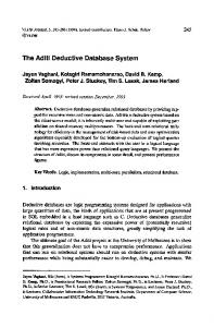
The tours must visit the named regions in the order in which they are given; all tours start and nish in Melbourne. We have two implementations of the code that nds trips (sequences of ights) between cities. One uses a daily schedule that associates the availability of ights with an absolute date; the other uses a weekly schedule that associates this information with days of the week, subject to seasonal restrictions. Airlines usually publish their schedules in the compact weekly format, but this format requires some processing before use. We have tested all four queries with both daily and weekly schedules, with the predicate nding trips between cities compiled with the magic set optimization and with the context transformation, and with the schedule relation being stored without indexing, with dynamic superimposed codeword indexing and with B-tree indexing. The keys used for indexing are the origin and destination cities together with the desired date of travel. The reason why we did not include data for the case when the trip- nding predicate is compiled without optimization is that that predicate is allowed only with respect to queries that specify the starting-date argument, and therefore the predicate cannot be evaluated bottom-up without rst being transformed by a magic-like optimization. The test results appear in tables 1 and 2, whose speedups are computed with respect to the magic transformed program using no indexing. Speedups for a given query follow the time and the colon. An M in the second column indicates that the magic set transformation was used, and a C in the second column indicates that the context transformation was used. The tables tell us several things. First, the context transformation consistently yields results 20% to 40% better than the magic set optimization. Second, the type of indexing has a signi cant impact only for the daily schedule, in which case the schedule relation contains 54,058 tuples. The four queries have 18, 12, 57 and 38 answers respectively. This is not apparent from the table due to two reasons. First, the tours with more answers are those that visit fewer regions and 10
Version
Query
Tour 1 Tour 2 Tour 3 Tour 4 M 381.1: 1.0 294.4: 1.0 360.2: 1.0 285.6: 1.0 C 282.3: 1.3 232.3: 1.3 266.5: 1.3 211.1: 1.3 Dsimc M 20.5: 18.6 16.9: 17.4 18.0: 20.0 14.2: 20.0 C 14.4: 26.5 11.7: 25.2 14.0: 25.7 11.7: 24.4 Btree M 17.5: 21.8 14.1: 20.9 15.4: 23.4 12.7: 22.5 C 13.9: 27.4 11.0: 26.7 13.5: 26.6 10.5: 27.1 Data
Table 1: Results for Phineas Fogg queries with daily schedule Version Data
M C Dsimc M C Btree M C
Tour 1 30.3: 1.0 24.3: 1.2 28.6: 1.1 21.4: 1.4 27.9: 1.1 23.2: 1.3
Query Tour 2 Tour 3 24.6: 1.0 28.2: 1.0 19.4: 1.3 23.0: 1.2 23.5: 1.0 25.3: 1.1 16.6: 1.5 20.7: 1.4 23.3: 1.1 26.1: 1.1 18.1: 1.3 22.0: 1.3
Tour 4 22.4: 1.0 17.8: 1.3 19.3: 1.2 15.1: 1.5 20.5: 1.1 16.8: 1.3
Table 2: Results for Phineas Fogg queries with weekly schedule thus call trip a smaller number of times. Second, the cost of the joins invoked by trip depend mostly on the sizes of the input relations and very little on the size of the output relation. As one expects, accessing such a large relation without an index has a large penalty, ranging from about 17-fold to about 24-fold. For these queries the trip predicate always speci es all three of the key arguments of the schedule relation, so B-tree indexing is as e�ective as it can be. Dsimc indexing yields slightly lower performance (by about 10% to 20%), mainly because dsimc uses the keys only to restrict its attention to a set of pages and cannot focus directly on the tuples of interest within those pages. For the weekly schedule, in which the relation contains 1,044 tuples, most of the time is spent in computation, not retrieval, and so the type of indexing makes little di�erence: there is less than 10% variation among all the numbers. The main sources of this variation are probably the di�erences between the overheads of the various indexing methods.
6 Conclusion We have described the implementation of a ights database system in Aditi. This was, in some ways, a test of the system to see how well it could be used for the development of an application. It was certainly adequate for this task, and our experience leads us to believe that deductive database technology is an excellent framework for the rapid development of complex systems. Some features of Aditi, in particular B-tree indexes, the ability to handle large amounts of data and support for function symbols, were crucial to the development of the system. This particular application also suggested the intermixing of top-down and bottom-up execution methods, which has been 11
incorporated into Aditi, and the use of set indexing methods. It is our belief that deductive database systems will need to be demonstrably impressive in order to gain commercial acceptance, and that a ights database, like the Aditi version of one described in this paper, is a good example of the application of techniques peculiar to deductive database systems. We have demonstrated this system to people interested in nding out more about deductive database systems, and the reaction has been generally quite positive. In particular, it is recognised that this is a realistic problem to which deductive databases are particularly suited, and one which is easily comprehended by the non-expert. In order to make the demonstrations run more smoothly, we have also developed a form of graphical output for queries, in that the actual
ight paths found by the system are drawn on a map of the world on the screen. Whilst such bells and whistles do not represent much original work, they appear to be virtually mandatory in order to attract the attention of the database community at large. The system has also been a useful test for Aditi. For example, the daily schedule, containing more than 54,000 tuples, has been a very useful test of the way that Aditi reacts under load, and of the implementation of the indexing methods. Whilst this particular application has been produced by the developers of Aditi, it seems that such a demonstration system is necessary in order to get others interested in using deductive database systems in a signi cant way. We are actively encouraging such interaction, as well as pursuing further Aditi applications.
7 Acknowledgements The assistance of the Key Centre for Knowledge Bases Systems, the Australian Research Council, the Co-operative Research Centre for Intelligent Decision Systems and the Collaborative Information Technology Research Institute is gratefully acknowledged.
References [1] I. Balbin, G. Port, K. Ramamohanarao and K. Meenakshi, E�cient Bottom-up Computation of Queries on Strati ed Databases, Journal of Logic Programming 11:295-345, 1991. [2] I. Balbin and K. Ramamohanarao, A Generalization of the Di�erential Approach to Recursive Query Evaluation, Journal of Logic Programming 4:259-262, 1987. [3] F. Bancilhon, D. Maier, Y. Sagiv and J. Ullman, Magic Sets and Other Strange Ways to Implement Logic Programs, Proceedings of the ACM Symposium on Principles of Database Systems 1-15, Cambridge, 1986. [4] C. Beeri and R. Ramakrishnan, On the Power of Magic, Proceedings of the ACM Symposium on Principles of Database Systems 269-283, San Diego, 1987. [5] D. Kemp, K. Ramamohanarao and Z. Somogyi, Right-, Left- and Multi-linear Rule Transformations which Maintain Context Information, Proceedings of the Sixteenth International Conference on Very Large Databases 380-391, Brisbane, August, 1990. [6] R. Ramakrishnan, D. Srivastava and S. Sudarshan, Rule Ordering in Bottom-up Fixpoint Evaluation of Logic Programs, Proceedings of the Sixteenth International Conference on Very Large Databases 359-371, Brisbane, August, 1990. 12
[7] D. Sacca and C. Zaniolo, Implementation of Recursive Queries for a Data Language Based on Pure Horn Logic, Proceedings of the Fourth International Conference on Logic Programming 104-135, Melbourne, May, 1987. [8] J. Vaghani, K. Ramamohanarao, D. Kemp, Z. Somogyi, P. Stuckey, T. Leask and J. Harland, The Aditi Deductive Database System, VLDB Journal 3:2:245-288, April, 1994.
13