Our algorithm has been implemented in the Matlab program besselint, which also works under Octave. For more information about the different versions of Mat-.
A Matlab Implementation of an Algorithm for Computing Integrals of Products of Bessel Functions Joris Van Deun and Ronald Cools Dept. of Computer Science, K.U. Leuven, B-3001 Leuven, Belgium {joris.vandeun, ronald.cools}@cs.kuleuven.be Abstract. We present a Matlab program that computes infinite range integrals of an arbitrary product of Bessel functions of the first kind. The algorithm uses an integral representation of the upper incomplete Gamma function to integrate the tail of the integrand. This paper describes the algorithm and then focuses on some implementation aspects of the Matlab program. Finally we mention a generalisation that incorporates the Laplace transform of a product of Bessel functions.
1 Introduction Integrals of products of Bessel functions arise in a wide variety of problems from physics and engineering. Many of the integrals that occur in the literature contain only one or two Bessel functions, e.g. in computing the filter loss coefficient in optical fibre technology [11], surface displacement in dynamic pavement testing [16], antenna theory [17], gravitational fields of astrophysical discs [5], crack problems in elasticity [22], particle motion in an unbounded rotating fluid [6,21], theoretical electromagnetics [8] or distortions of nearly circular lipid domains [20]. Techniques to compute this type of integrals are discussed in [2,14,22]. Analytic expressions for some special cases can be found in [19,26]. The more general case of a product of an arbitrary number of Bessel functions is far more difficult to handle and there are less analytic results known. For three or four factors we refer to [15,19,26]. The last reference also contains examples of integrals with an arbitrary number of factors. The numerical computation of these integrals has not gained much attention, even though they occur in several applications, ranging from Feynman diagrams in nuclear physics [10] to quantum field theory [7], speech enhancement [13] and scattering theory [9]. In [25] we presented an algorithm to compute integrals of the form � ∞ k � m x Jνi (ai x)dx (1) I(a, ν, m) = 0
i=1
(we use a to denote the vector which contains these where the coefficients ai ∈ � coefficients), the orders νi ∈ R, the power m ∈ R and ki=1 νi + m > −1. This last condition assures that a possible singularity in zero is integrable. However, if some of the νi are negative integers, this condition may not be satisfied, even though the integral exists. This follows from formula 9.1.5 in [1] which reads as follows, R+ 0
J−n (x) = (−1)n Jn (x). A. Iglesias and N. Takayama (Eds.): ICMS2006, LNCS 4151, pp. 284–295, 2006. c Springer-Verlag Berlin Heidelberg 2006 �
A Matlab Implementation of an Algorithm
285
This case is detected by the program and the formula is used to transform negative integer orders to positive integer orders. The case of negative coefficients ai can always be reduced to the case of positive coefficients using [1, p. 360] Jν (−z) = eνπi Jν (z), where i is the imaginary unit, i2 = −1. We leave it to the user to do this transformation, so that the output of our program is always a real number. Our algorithm has been implemented in the Matlab program besselint, which also works under Octave. For more information about the different versions of Matlab and Octave we tested, we refer to the section about backward compatibility. We also mention that our program solves one of the additional problems arising from Trefethen’s 100-Digit Challenge [23]. Problem 8 in Appendix D of the book [4] concerns the evaluation of the integral � ∞ √ √ √ √ √ xJ0 (x 2)J0 (x 3)J0 (x 5)J0 (x 7)J0 (x 11)dx, (2) 0
which is just a special case of the more general formula (1). In the next section we describe how the algorithm works. In the rest of the paper we then discuss some implementation issues particularly related to the fact that the program is meant to be used under Matlab or Octave and we mention some possible improvements and generalisations.
2 Description of the Algorithm We provide a brief overview of the algorithm. For more details we refer the reader to [25]. The main difficulties in computing (1) come from the irregular oscillatory behaviour and possible slow decay of the integrand. We cannot just truncate the integral at a finite value and assume that the remaining contribution is negligible; the infinite part needs special treatment. This is illustrated in Figures 1 and 2, which show the integrand of formula (2). The approach we take is to split the integral at a breakpoint x0 and approximate the finite and infinite part separately. The determination of this breakpoint will be discussed below. For the finite part, the interval [0, x0 ] is divided into a number of subintervals roughly proportional to the number of zeros in the integrand. Each subinterval is then integrated numerically using a Gauss-Legendre quadrature rule. The weights and nodes have been hard-coded into the program to speed up performance. In most cases we need a 15–point rule to reach full precision, followed by a 19–point rule to obtain the error estimate. From formula 9.1.7 in [1] it follows that the integrand f (x) satisfies f (x) = xp
∞ � i=0
αi xi ,
x → 0,
286
J. Van Deun and R. Cools
0.2 0.15 0.1 0.05 0 −0.05 0
0.5
1
1.5
2
Fig. 1. Plot of the integrand of formula (2) near x = 0
� (the exact values of αi are not relevant), where p = ki=1 νi + m. If p is not a positive integer, there is an algebraic singularity in 0 which we can remove by extrapolating in the sense of Richardson. This has also been incorporated in the program. For the infinite part we use the asymptotic expansion of Jν (x) as given in [26, p. 199]. Taking n + 1 terms in each expansion leads to an approximation of the form ⎧ ⎫ k ⎨ � ⎬ � Jνi (ai x) ∼ 2� xm eiηj x Fn,j (ν, ax) xm ⎩ ⎭ i=1
j
where � denotes the real part, ηj = a1 ± a2 ± · · · ± ak and the sum is over all possible combinations. The functions Fn,j consist of polynomials of degree k(2n + 1) in 1/x times x−k/2 . Integrating this approximation, we have to compute � ∞ eiηi x xm−k/2−j dx, i = 1, 2, . . . , 2k−1 , j = 0, 1, . . . , k(2n + 1). (3) x0
which we can do analytically, using the upper incomplete Gamma function. This function is defined as [1, p. 260] � ∞ Γ (a, x) = ta−1 e−t dt, x
and can be extended to arbitrary complex a and x by analytic continuation. This way we may write �
∞
x0
eiηi x xm−k/2−j dx =
i ηi
m−k/2−j+1 Γ (m − k/2 − j + 1, −iηi x0 ).
(4)
The accuracy of the approximation for the infinite part depends on the breakpoint x0 and on the order of the asymptotic expansion n, and we can estimate this accuracy
A Matlab Implementation of an Algorithm
287
0.002 0.001 0 −0.001 −0.002 −0.003 0
5
10
15
20
Fig. 2. Plot of the tail of the integrand of formula (2)
(as a function of x0 and n) based on a first order error analysis. It then turns out that for a fixed accuracy there are always infinitely many (x0 , n)-pairs we can choose from. We therefore introduced a cost function χ(x0 , n) which describes the computational effort of the algorithm in terms of the number of function evaluations of the Bessel and incomplete Gamma functions, χ(x0 , n) = 2k ntGJ +
k x0 N � aj . π 2 j=1
The parameter N is the average length of the vector argument in a call to the Bessel function. This will be explained in the next section. The (machine-dependent) constant tGJ is the relative efficiency of computing the incomplete Gamma function compared to computing the Bessel function. We look at this constant in more detail in the next section. The parameters x0 and n are now chosen such that they minimise χ(x0 , n) under the constraint that the (estimated) error does not exceed a required threshold. It is up to the user to specify the absolute or relative error tolerance.
3 Determining the Parameter tGJ When introducing the cost function χ(x0 , n), we assumed that the computational effort is dominated by the evaluations of the Bessel and incomplete Gamma function. In our program, we use Matlab’s besselj function, based on Amos’ original Fortran code [3], to compute the Bessel functions. For the incomplete Gamma function we use igamma, a Fortran-to-Matlab conversion of the program from [12], which computes a continued fraction approximation by forward recurrence. To test the assumption that the cost is dominated by these two functions, we run besselint on a set of 21 examples which are thought to be representative (in the sense that they do not use extremely large values for the parameters or the number of factors in the integrand). The values of a,
288
J. Van Deun and R. Cools
Table 1. Values of a, ν, m and I(a, ν, m) for the examples from the test set. If more than 10 digits are shown, then the least significant one is properly rounded; otherwise the given value is exact a
ν
m I(a, ν, m)
1
1
2
1
1 3 − 14
3
1
0
2 −1
4
1
0
4 9
5
[1, 5]
[0, 1]
0 0.2
6
[5, 1]
[0, 1]
0 0
7
[1, 3]
8
[3, 1] √ √ √ [ 2, 3, 5] √ √ √ [ 2, 3, 11] √ √ √ [ 2, 3, 5] √ √ √ [ 2, 3, 5] √ √ √ [ 2, 3, 11] √ √ √ √ [ 2, 3, 5, 7]
9 10 11 12 13 14
[− 12 [− 12
0 1 1 3
1 ] 3 1 ] 3
1 6 1 6
0
0.4699242939646020
0.4875332490256343 0
1 0.1299494668722794
0
1 0
1
0 0.1423525086834354
[1, 2, −3]
1 −0.1150621628914800
[1, 2, −3]
1 0
0
1 0.1104110282210471
[1, 1, 1, 1] √ √ √ √ √ 16 [ 2, 3, 5, 7, 11] √ √ √ √ √ 17 [ 2, 3, 5, 7, 11]
5 4
− 32 0.05133002738452328
0
1 0.06106434990872167
18
[8, 2.5, 2, 1.5, 1]
1
19
[8, 2.5, 2, 1.5, 1, 0.5]
20
[1, 2, 3] √ √ √ √ [ 2, 3, 2 + 3]
15
21
0 [ 13 −
1 4
−
1 4
−
2 0.017024879933914 −2 0 1 4
−
1 4
− 14 ]
7 12
0.5219234259420822
0
0 0.4752701735935373
0
0 0.4437109037960439
ν and m for each of the examples, together with the value of the integral, are given in Table 1. For tGJ we take the value 16, for reasons explained below. We used Matlab’s profiler tool to analyse the distribution of CPU time among the various subfunctions in besselint (the main program which contains the 21 calls to besselint is called experiment, which is the first line in the profiler report). Table 2 reproduces the output report provided by the profiler. Computations were done in Matlab 7.0 on an Intel processor running at 2.80 GHz. Note that besselj and igamma together take up 3.45s of the total 4.53s of execution time, which is more than 76%. It seems our assumption is justified. As we mentioned in the previous section, the parameter tGJ is the relative efficiency of computing the incomplete Gamma function compared to computing the Bessel function. It is defined as the ratio tΓ /tJ where tΓ and tJ are the average execution times for a call to the incomplete Gamma function and Bessel function respectively. The determination of this parameter, however, presents some problems which we discuss next.
A Matlab Implementation of an Algorithm
289
Table 2. Matlab’s profiler output after calling besselint with the test set Profile Summary Generated 21-Oct-2005 13:10:04 using CPU time. Function Name experiment besselint besselint>fri besselint>nqf besselint>fun besselj besselint>ira igamma igamma>cdh igamma>cdhs besselmx (MEX-function) besschk besselint>gop besselint>optimfun besselint>auxfun conv gammaln repmat datenummx (MEX-function) profile>ParseInputs
Calls 1 21 21 66 1343 5470 21 2027 2027 2027 5470 5470 21 84 84 464 252 21 2 1
Total Time 4.530 s 4.490 s 2.710 s 2.670 s 2.360 s 2.180 s 1.570 s 1.270 s 1.190 s 1.130 s 0.820 s 0.590 s 0.150 s 0.100 s 0.100 s 0.010 s 0.050 s 0.010 s 0s 0s
Self Time 0.040 s 0.060 s 0.040 s 0.310 s 0.180 s 0.770 s 0.280 s 0.080 s 0.060 s 1.130 s 0.820 s 0.590 s 0.050 s 0.000 s 0.050 s 0.010 s 0.050 s 0.010 s 0.000 s 0.000 s
Self time is the time spent in a function excluding the time spent in its child functions. Self time also includes overhead resulting from the process of profiling.
The first problem in determining tGJ comes from the fact that Matlab and Octave support vector operations. This means that we can call the function besselj with a vector argument to evaluate the Bessel function in N points at the same time. This will generally be faster than N separate calls. Obviously, we exploited this in our program. This has to be taken into account when trying to determine tJ . To determine tGJ we timed 2040 calls to igamma and 120 calls with a vector argument of length 17 = 2040/120 to besselj (for most representative examples, an average call to besselj in the numerical quadrature formula would contain a vector of this size). Averaging over 22 runs gives a ratio of more or less tGJ ≈ 16 in Matlab 7.0 and tGJ ≈ 1357 in Octave 2.1.69. Another problem comes from the fact that our cost function is not exact. Even though it is clear that the dominant contribution to the computational effort comes from evaluating the incomplete Gamma function and the Bessel function, the other operations are not negligible. Apart from all this, it needs pointing out that the Matlab compiler and JIT (Just In Time) accelerator have become so sophisticated that it becomes nearly impossible to minimise execution times based on operation count. To illustrate this discussion
290
J. Van Deun and R. Cools
0.18
time (s)
0.17 0.16 0.15 0.14 0.13 0
10
20
30
40
50
tGJ Fig. 3. Average execution time (s) for a call to besselint vs. tGJ (Matlab)
we run besselint on the previous set of 21 examples, but this time for different values of tGJ . Averaging over 10 runs gives the results from Figures 3 and 4. These figures give the average execution time for one (representative) call to besselint as a function of the parameter tGJ . It can be seen that the predicted ‘theoretical’ values of tGJ differ from the experimentally determined ‘optimal’ values. For the Matlab case, the difference in execution time is small, but if speed is a real concern, the user might want to repeat this test on his own machine to obtain the optimal tGJ . Note that our code runs much faster under Matlab than under Octave. It is not clear what causes this difference.
4 Backward Compatibility Our program was written to work in Matlab 7.0 and Octave 2.1.69. However, we specifically implemented it to be backward compatible with earlier versions of Matlab. Especially for a large commercial software package such as Matlab, one cannot simply assume that every user has access to the latest available version. We extensively tested our code under – – – –
Matlab 7.0.1.24074 (R14) Service Pack 1 for Linux, Matlab 6.5.0.180913a (R13) for Linux and Windows, Matlab 6.1.0.450 (R12.1) for Windows, and Octave 2.1.69.
However, improving backward compatibility usually means losing some efficiency. This is particularly true when it comes to logical operations in Matlab, as we illustrate in this section.
A Matlab Implementation of an Algorithm
291
2.5
time (s)
2
1.5
1
0.5 0
200
400
600
800
1000
tGJ Fig. 4. Average execution time (s) for a call to besselint vs. tGJ (Octave)
Logical expressions such as x ∨ y (where x and y are booleans and ∨ is the logical ‘or’) are very common in numerical software and they very often appear in conditional statements to control the flow of a program. For both the logical ‘or’ and ‘and’ there are situations where only one of the operands needs to be evaluated to determine the result. For example, in the expression x ∨ y, if x is ‘true’, the result will be ‘true’ regardless of the value of y. In Matlab terminology, this is called ‘short-circuit’ logical evaluation. When there are many logical expressions in a program, this can be much more efficient than evaluating the entire expression (called ‘element-wise’ evaluation in Matlab). Unfortunately, there is a difference in syntax between earlier and recent versions of Matlab. From version 6.5 on, Matlab explicitly provides two different sets of logical operators, i.e. element-wise operators denoted by & and |, and short-circuit operators, && and || (which is also the convention used by Octave from the beginning). However, in earlier versions of Matlab, the explicit short-circuit operators were not available and short-circuit evaluation was done automatically in certain situations (e.g. in the condition following an if-statement). Because of backward compatibility, we have to use the operators & and |, which dramatically reduces efficiency when working in more recent versions. Table 3 was obtained in exactly the same way as Table 2, but with the only difference that all logical operators were replaced by their short-circuit versions. The total execution time for the test examples has changed from 4.69s to 3.93s, a reduction of over 13%, but if we compare the timings for igamma, then we note a reduction from 1.27s to 0.6s, more than 50%! The number of incomplete Gamma function evaluations increases exponentially with k (the number of Bessel functions in the integrand), so especially for integrals which contain many Bessel functions, we are sacrificing a lot of efficiency to the cause of backward compatibility. We do not know why Mathworks decided to introduce this syntactic anomaly for logical operators.
292
J. Van Deun and R. Cools Table 3. Same as Table 2, but using short-circuit logical evaluation Profile Summary Generated 21-Oct-2005 13:53:21 using CPU time. Function Name experiment besselint besselint>fri besselint>nqf besselint>fun besselj besselint>ira besselmx (MEX-function) besschk igamma igamma>cdh igamma>cdhs besselint>gop besselint>optimfun besselint>auxfun gammaln conv repmat datenummx (MEX-function) profile>ParseInputs
Calls 1 21 21 66 1343 5470 21 5470 5470 2027 2027 2027 21 84 84 252 464 21 2 1
Total Time 3.930 s 3.860 s 2.620 s 2.590 s 2.230 s 2.050 s 0.980 s 0.820 s 0.690 s 0.600 s 0.500 s 0.410 s 0.190 s 0.170 s 0.160 s 0.080 s 0.030 s 0.010 s 0s 0s
Self Time 0.070 s 0.070 s 0.030 s 0.360 s 0.180 s 0.540 s 0.340 s 0.820 s 0.690 s 0.100 s 0.090 s 0.410 s 0.020 s 0.010 s 0.080 s 0.080 s 0.030 s 0.010 s 0.000 s 0.000 s
Self time is the time spent in a function excluding the time spent in its child functions. Self time also includes overhead resulting from the process of profiling.
5 Further Improvements and Generalisations The function besselj essentially consists of two function calls, one to besschk, which checks the input arguments, and then a call to besselmx, which is a MEX file containing the actual Amos algorithm to compute Jν (x). According to the profiler report, both calls take up approximately 40% of the total time for this function. Since the arguments to the Bessel functions are computed inside besselint and are not given by the user, this means we could speed up performance by calling besselmx directly instead of besselj, thereby skipping the call to besschk. This effectively reduces the computation time for besselj from 2.18s to 0.78s for besselmx (backward compatible version). Also the overhead associated with function calls is reduced. The problem with this approach, however, is that it only works in Matlab and not in Octave, which uses a different implementation. Since we want to provide a program that works both under Matlab and Octave, we have not performed this optimisation. For the other bottleneck, igamma, there are two things we can do to speed up the computations. The most obvious improvement is to compute the continued fraction approximation by backward recurrence instead of forward, which is usually faster and also more stable. However, then we need a good estimate of the tail to be able to predict
A Matlab Implementation of an Algorithm
293
at what point to start the recurrence. The formulas from [27] are useless in our case, because they give asymptotic estimates which only become valid when extremely high precisions (working in multiprecision) are needed. In a Matlab environment, which uses IEEE double precision, they give unreliable results.
Relative error of Γ(x − j, iy)
10−6
10−9
10−12
10−15 10
20
30
40
50
60
j Fig. 5. Error in recurrence for Γ (x − j, iy) for x = −1, j = 0, . . . , 60 and y = 25. The solid line shows the relative error when the recurrence is computed starting from the value at the left and going to the right, the dashed line corresponds to going from right to left.
The second improvement to igamma comes from the recurrence relation satisfied by this function itself. Looking at equations (3) and (4), we see that a range of incomplete Gamma function evaluations are needed of the form Γ (x − j, iy),
j = 0, 1, . . . , s
for certain values of x, y and s. But it follows from [1], formulas 6.5.2, 6.5.3 and 6.5.21 that we have Γ (x − j + 1, iy) = (x − j)Γ (x − j, iy) + (iy)x−j e−iy . So instead of evaluating the incomplete Gamma function 2k−1 (k(2n + 1) + 1) times using the continued fraction expansion, we could suffice with 2k−1 evaluations and compute the remaining values recursively. However, it turns out that for several values of x and y, this recurrence can become unstable in either direction. This means we can loose (too many) digits both using forward or backward recurrence (of course, it will be asymptotically stable in one direction, but that is of little use when we want all values to have maximum precision). This is illustrated in Figure 5, which shows the relative error as a function of j for x = −1, y = 25 and s = 60. The correct approach here is to find the value of j for which the error reaches its maximum value (in our example
294
J. Van Deun and R. Cools
j ≈ 24) and then use the recurrence relation in both directions, starting from that point. This is explained in more detail in [24]. Instead of using the continued fraction expansion to compute the incomplete gamma function, another possibility would be to use asymptotic expansions (at least when one or both of the parameters are large). Since no such implementation is available and since the computation of the incomplete gamma function was not our main concern, we have not yet considered this. The present algorithm can be generalised to compute integrals of the form � 0
∞
e−cx
k xm � Jν (ai x)dx 1 + dx2 i=1 i
where c is a positive real number and d is an arbitrary real number. The case d = 0 corresponds to the Laplace transform of a product of Bessel functions. Integrals of this type occur in several applications, e.g. in [18]. This generalisation, however, is not so straightforward (especially when d = 0) and the details will be presented elsewhere.
6 Conclusion In the development of numerical software there is often a tradeoff to be made between speed and efficiency on the one hand, and compatibility on the other hand. We wanted to provide an implementation of our algorithm that works for older versions of Matlab and for Octave as well, but the experiments in this article clearly indicate that we can gain a lot of speed with a program that only runs under recent versions of Matlab. Based on our timings, we expect that it is possible to obtain an implementation which is (on average) roughly twice as fast as the current one. However, more research needs to be done regarding the recursive computation of the incomplete Gamma function. Theoretically, the approach presented in [24] should work fine, but a robust implementation has not yet been undertaken.
References 1. M. Abramowitz and I. A. Stegun. Handbook of Mathematical Functions With Formulas, Graphs, and Mathematical Tables, volume 55 of Applied Mathematics Series. National Bureau of Standards, Washington, D.C., 1964. 2. V. Adamchik. The evaluation of integrals of Bessel functions via G–function identities. J. Comput. Appl. Math., 64:283–290, 1995. 3. D. E. Amos. Algorithm 644: A portable package for Bessel functions of a complex argument and nonnegative order. ACM Trans. Math. Software, 12(3):265–273, 1986. 4. F. Bornemann, D. Laurie, S. Wagon, and J. Waldvogel. The SIAM 100-Digit Challenge. A Study in High-Accuracy Numerical Computing. SIAM, Philadelphia, 2004. 5. J. T. Conway. Analytical solutions for the newtonian gravitational field induced by matter within axisymmetric boundaries. Mon. Not. R. Astron. Soc., 316:540–554, 2000. 6. A. M. J. Davis. Drag modifications for a sphere in a rotational motion at small non-zero Reynolds and Taylor numbers: wake interference and possible coriolis effects. J. Fluid Mech., 237:13–22, 1992.
A Matlab Implementation of an Algorithm
295
7. S. Davis. Scalar field theory and the definition of momentum in curved space. Class. Quantum Grav., 18:3395–3425, 2001. 8. G. Fikioris, P. G. Cottis, and A. D. Panagopoulos. On an integral related to biaxially anisotropic media. J. Comput. Appl. Math., 146:343–360, 2002. 9. R. Gaspard and D. Alonso Ramirez. Ruelle classical resonances and dynamical chaos: the three- and four-disk scatterers. Physical Review A, 45(12):8383–8397, 1992. 10. S. Groote, J. G. K¨orner, and A. A. Pivovarov. On the evaluation of sunset-type Feynman diagrams. Nucl. Phys. B, 542:515–547, 1999. 11. M. J. Holmes, R. Kashyap, and R. Wyatt. Physical properties of optical fiber sidetap grating filters: free space model. IEEE Journal on Selected Topics in Quantum Electronics, 5(5):1353–1365, 1999. 12. E. Kostlan and D. Gokhman. A program for calculating the incomplete Gamma function. Technical report, Dept. of Mathematics, Univ. of California, Berkeley, 1987. 13. T. Lotter, C. Benien, and P. Vary. Multichannel direction-independent speech enhancement using spectral amplitude estimation. EURASIP Journal on Applied Signal Processing, 11:1147–1156, 2003. 14. S. K. Lukas. Evaluating infinite integrals involving products of Bessel functions of arbitrary order. J. Comput. Appl. Math., 64:269–282, 1995. 15. J. W. Nicholson. Generalisation of a theorem due to Sonine. Quart. J. Math., 48:321–329, 1920. 16. J. M. Roesset. Nondestructive dynamic testing of soils and pavements. Tamkang Journal of Science and Engineering, 1(2):61–81, 1998. 17. S. V. Savov. An efficient solution of a class of integrals arising in antenna theory. IEEE Antenna’s and Propagation Magazine, 44(5):98–101, 2002. 18. N. P. Singh and T. Mogi. Electromagnetic response of a large circular loop source on a layered earth: a new computation method. Pure Appl. Geophys., 162:181–200, 2005. 19. N. J. Sonine. Recherches sur les fonctions cylindriques et le d´eveloppement des fonctions continues en s´eries. Math. Ann., 16:1–80, 1880. 20. H. A. Stone and H. M. McConnell. Hydrodynamics of quantized shape transitions of lipid domains. Royal Society of London Proceedings Series A, 448:97–111, 1995. 21. J. Tanzosh and H. A. Stone. Motion of a rigid particle in a rotating viscous flow: an integral equation approach. J. Fluid Mech., 275:225–256, 1994. 22. M. Tezer. On the numerical evaluation of an oscillating infinite series. J. Comput. Appl. Math., 28:383–390, 1989. 23. L. N. Trefethen. The $100, 100-Digit Challenge. SIAM News, 35(6):1–3, 2002. 24. J. Van Deun and R. Cools. A stable recurrence for the incomplete Gamma function with imaginary second argument. Technical Report TW441, Department of Computer Science, K.U.Leuven, November 2005. 25. J. Van Deun and R. Cools. Algorithm 8XX: Computing infinite range integrals of an arbitrary product of Bessel functions. ACM Trans. Math. Software, 2006. To appear. 26. G. N. Watson. A treatise on the Theory of Bessel Functions. Cambridge University Press, 1966. 27. S. Winitzki. Computing the incomplete Gamma function to arbitrary precision. In V. Kumar, M. L. Gavrilova, C. J. K. Tan, and P. L’Ecuyer, editors, Computational Science and Its Applications – ICCSA, volume 2667 of Lecture Notes in Computer Science, pages 790–798. Springer Verlag, 2003.