AN ALGEBRAIC MULTIGRID METHOD FOR LINEAR ... - CiteSeerX

AN ALGEBRAIC MULTIGRID METHOD FOR LINEAR ELASTICITY MICHAEL GRIEBEL† ‡ , DANIEL OELTZ‡ AND MARC ALEXANDER SCHWEITZER† Abstract. We present an algebraic multigrid (AMG) method for the efficient solution of linear (block-)systems stemming from a discretization of a system of partial differential equations (PDEs). It generalizes the classical AMG approach for scalar problems to systems of PDEs in a natural blockwise fashion. We apply this approach to linear elasticity and show that the block-interpolation, described in this paper, reproduces the rigid body modes, i.e., the kernel elements of the discrete linear elasticity operator. It is well-known from geometric multigrid methods that this reproduction of the kernel elements is an essential property to obtain convergence rates which are independent of the problem size. We furthermore present results of various numerical experiments in two and three dimensions. They confirm that the method is robust with respect to variations of the Poisson ratio ν. We obtain rates ρ < 0.4 for ν < 0.4. These measured rates clearly show that the method provides fast convergence for a large variety of discretized elasticity problems. Key words. algebraic multigrid, system of PDEs, linear elasticity AMS subject classifications. 65N55, 65N22, 65F10

1. Introduction. The solution of large sparse linear systems is an essential ingredient in most scientific computations. The ever growing demand for efficient solvers led to the development of geometric multigrid methods in the 1970’s [2, 3, 14, 15]. But for many applications it is difficult to construct a sequence of (nested) discretizations or meshes needed for geometric multigrid. Furthermore, geometric multigrid methods are in general not robust with respect to a deterioration of the coefficients of the operator or singular perturbations. In the 1980’s algebraic multigrid (AMG) methods were developed [4, 6, 8, 9, 18] to cope with these problems by extending the main ideas of geometric multigrid methods to a purely algebraic setting. This approach is based only on information available from the linear system to be solved. These methods can be applied successfully to many linear systems which come from a discretization of a scalar (elliptic) partial differential equation (PDE) [12, 13, 20]. But in the case of systems of PDEs most of the AMG methods fail. In this paper we present a generalization of classical AMG to systems of PDEs where we assume only that the linear system is provided in point-block-form, i.e., all couplings between the unknowns corresponding to a particular node of the discretization make up a local block of the system matrix. Then, the so-called point-block approach, which was first proposed by Brandt [5], defines in a natural way the restriction and prolongation operators in a blockwise fashion. Here, a block-prolongation operator based on a basic interpolation scheme and standard coarse grids leads to the exact interpolation of the kernel elements of the linear elasticity operator. Furthermore, this main theoretical result shows that classical AMG concepts can successfully be applied to the system case and no modifications such as smoothed aggregation [22] or other techniques are necessary to obtain fast convergence. The remainder of the paper is organized as follows: In section 2 we give a short † Sonderforschungsbereich 611, Singul¨ are Ph¨ anomene und Skalierung in mathematischen Modellen, Institut f¨ ur Angewandte Mathematik, Universit¨ at Bonn, Wegelerstr. 6, D-53115 Bonn, (griebel, schweitz)@iam.uni-bonn.de ‡ Sonderforschungsbereich 408, Anorganische Festk¨ orper ohne Translationssymmetrie, Institut f¨ ur Angewandte Mathematik, Universit¨ at Bonn, Wegelerstr. 6, D-53115 Bonn, (griebel, oeltz)@iam.unibonn.de

1

review of the (scalar) AMG algorithm and the respective heuristics, which led to its development. Then, we present the two main difficulties which classical AMG can encounter in the systems case. These two issues can be overcome with the help of our generalized (point-block-)AMG approach which we present in section 3. As a main result, we prove in section 3.3 the exact interpolation of the kernel elements of the linear elasticity operator, the rigid body modes, which is, as for any multigrid algorithm, a fundamental property for the convergence behavior of the method. In section 4, we present the results of our numerical experiments with the point-blockAMG method for discretizations from linear elasticity. We focus on the stability of the method with respect to the mesh-width as well as on the robustness with respect to the Poisson ratio ν. Here, we also consider discretizations on complex geometries and unstructured grids. Finally, we conclude with some remarks in section 5. 2. Algebraic Multigrid Methods for Scalar PDEs. In this section we give a short review of the basic algebraic multigrid algorithm (for scalar PDEs) and the heuristics which led to its development, see [20] for a detailed introduction to AMG. Algebraic multigrid methods were first introduced in the early 1980’s [4, 6, 8, 9, 18] for the solution of linear systems Au = f coming from the discretization of scalar elliptic PDEs. The development of AMG was led by the idea to mimic (geometric) multigrid methods, i.e. their functionality and convergence behavior, in applications where a hierarchy of (nested) meshes and interlevel transfer operators could not (or only with huge effort) be provided. The amount of input information for the iteration scheme should be minimal, i.e., the linear system itself should provide all the information needed for the algorithm. In any multigrid method we devise two components which work on different parts of the spectrum of the (discrete) operator A, namely the smoother and the coarse grid correction, to reduce all error components in the overall iteration. Here, the coarse grid correction itself (i.e. its quality) is dependent on two ingredients: The coarse grid selection and the design of appropriate prolongation operators which are used to transfer information between the grids (i.e. the function spaces). In geometric multigrid methods the freedom in the selection of the coarse grid is somewhat limited. We usually deal with nested grids which are uniformly coarsened or semi-coarsened. In any case the sequence of grids is constructed based on information other than the system matrix A. The coarse grids are usually part of the discretization process itself. Either they come from an earlier, less accurate discretization of the continuous problem or they are constructed by means of geometric information and a-priori knowledge about the continuous problem and its solution. Here, the coarse grids are designed in such a way that (geometrically) smooth functions can be represented accurately on the coarser grids. In algebraic multigrid we have (in general) no access to the geometry of the problem or even the continuous problem itself. Here, we have to devise the smoother, the coarse grids and the transfer operators based only on information we can get from the linear system itself, i.e. from the discrete operator. Hence, we already lack the notion of (geometrically) smooth functions which could be used to design coarser grids. Therefore, we have to generalize the concept of geometric smoothness to some measurable quantity which can be (easily) computed from the discrete operator itself. Several different measures for the so-called algebraic smoothness are used today in the various algebraic multigrid methods developed over the years. Common to all these heuristic definitions is the general observation that a simple relaxation scheme— most often Gauß–Seidel smoothing is used in AMG—damps (efficiently) high energy 2

components, i.e. eigenvectors associated with large eigenvalues, only. Consequently, the coarse grid correction must be able to deal with the remaining small energy components. These small energy functions should be represented accurately on coarser grids. Some of the characterizations for such small energy components e are: 1) Ae ' 0, 2) hAe, ei ' 0, 3) Ae = λe, with λ ' 0. In the classical AMG [18] approach 1) and in the element-based AMGe [10] criterion 2) is used for the characterization of smooth error, whereas in the spectral version of AMGe [11] 3) characterizes smooth components. Also Brandt’s compatible relaxation [7] can be used to define an appropriate coarse grid selection. 2.1. Coarsegrid Selection. Based on such an algebraic smoothness measure we can now introduce the notion of strong couplings between unknowns. For fixed 0 ≤ α ≤ 1 and the index set N := {1, ..., n} of all unknowns, an unknown i is said to be strongly coupled to an unknown j if |aij | ≥ α · maxk∈N |aik |. We define Si := {j | |aij | ≥ α · maxk∈N |aik |} as the set of all unknowns j to which i is strongly coupled and SiT as the set of all points which are strongly coupled to i, i.e. j ∈ SiT if i ∈ Sj . F ⊂ N is the set of all unknowns on the fine grid which are not on the coarse grid while C ⊂ N is the set of all coarse grid unknowns. Note that for scalar problems one can uniquely map the index i to the geometric grid point xi , where the ith basis function of the discretization is nonzero on the grid point xi . For the ease of notation we sometimes refer to a grid point xi or the associated unknowns simply by the respective index i. Finally, we need the auxiliary sets Ni := {j | aij 6= 0}, Ci := C ∩ Ni and Fi := F ∩ Ni . With these definitions we can introduce the first step of the coarse grid selection [13, 17], the setup phase one. Algorithm 1 (Setup Phase 1). 1. Set C = ∅ and F = ∅ 2. While C ∪ F 6= N do Pick i ∈ N \ (C ∪ F ) with maximal |SiT | + |SiT ∩ F | If |SiT | = 0 then set F = N \ C else set C = C ∪ {i}, F = F ∪ (SiT \ C) Note that the Setup Phase 1 does not guarantee that each point i in F is strongly coupled to a coarse grid point j ∈ C, which can lead to less effective coarse grids. Hence, we employ a second setup phase, which updates the coarse grid selection from phase 1 in an appropriate fashion, see [12] for details. To this end, we define the measure X ¢−1 ¡ d(i, I) := γ |aij |, where γ := max |aik | k∈Ni

j∈I

and I is any subset of N . Algorithm 2 (Setup Phase 2). 1. Set T = ∅ 2. While T ⊂ F do Pick i ∈ F \ T and set T = T ∪ {i} Set C˜ = ∅, Ci = Si ∩ C and Fi = Si ∩ F While Fi 6= ∅ do 3

Pick j ∈ Fi and set Fi = Fi \ {j} If d(j, Ci )/d(i, {j}) ≤ β then ˜ =0 If |C| Set C˜ = {j} and Ci = Ci ∪ {j} else Set C = C ∪ {i} and F = F \ {i} and Goto 2 endif endif Set C = C ∪ C˜ and F = F \ C˜ 2.2. Prolongation. For scalar elliptic PDEs of second order we usually have the constant function in the kernel of the continuous operator. Note that in the classical AMG [18] we assume that the constant vector is the discrete representation of the constant function. Hence, there is essentially a single constraint we have to respect in the construction of the interpolation P operator I = (wij ): Constant vectors should be interpolated exactly, i.e., the sum j wij of the weights of the interpolation operator I must equal one for all i.1 But this simple scheme does not provide satisfactory results for non M-matrices. More involved interpolation schemes like the so-called standard interpolation scheme due to St¨ uben [20] improve the robustness of the method with respect to non M-matrices. Here, the characterization 2) of the algebraic smooth error, Ae ' 0, is used to define the so-called direct interpolation [20] I D . For a given fine grid point i the direct interpolation I D yields P X ( j∈Ni aij ) X D P aij ej (2.1) wij ej = − (IF C eC )i = aii · j∈Pi aij j∈Pi

j∈Pi

for a fine grid point i ∈ F , where Pi ⊂ C is some appropriately chosen set of interpolation nodes and the subscripts C and F denote the indices of the coarse and fine grid points respectively. Here, we use Pi := C ∩ Si . This scheme however provides good results only if the set Pi = C ∩ Si is large enough, which is not guaranteed by the coarsening algorithm. Therefore, St¨ uben proposed the standard interpolation I S which employs the modified weights w ˜ij given by P X ( j∈Ni a ˜ij ) X S P a ˜ij ej , (2.2) w ˜ij ej = − (IF C eC )i = ˜ij a ˜ii · j∈Pi a j∈Pi

j∈Pi

where Pi := {j | j ∈ Ci or ∃k ∈ Si : j ∈ Ck }. Here, we compute the new coefficients P a a ˜ijPby replacing ej for all j ∈ Si \ C in the equation j∈Ni ij ej = 0 by ej = − k∈Nj ajk ek /ajj . Even though such sophisticated interpolation schemes widen the area of application for scalar AMG, the convergence of a scalar AMG method may still break down in the systems case. 2.3. Scalar AMG and Systems of PDE. One reason for the deterioration or break down of the convergence of classical AMG in the systems case is the coarsening process of scalar AMG methods. This process can lead to different coarse grids for the different physical unknowns, although all unknowns were discretized on the same (fine) grid. Even worse, coarse grids from scalar AMG coarsening can consist of 1 Smoothed aggregation AMG [21, 22] allows for the prescription of the functions, i.e. vectors, which should be interpolated accurately on coarser grids.

4

only one physical unknown. The second reason is the interpolation of scalar AMG. The quality of interpolation of the kernel elements of the continuous operator plays a fundamental role for the convergence of the AMG method. For scalar elliptic problems the kernel of the continuous operator contains only constant functions represented by a constant vector. Therefore the condition that the sum of the interpolation weights equals one suffices to reproduce exactly these constant elements in the case of zero row sum matrices. In the system case, however, the kernel of the continuous operator generally contains more elements than constant scalar functions and the condition on the row sum of the interpolation operator given above does no longer lead to the exact interpolation of the kernel elements. One approach to overcome these issues is the so-called point-block approach which we present in the next section. 3. Algebraic Multigrid Methods for Systems of PDEs. We now present the generalization of the scalar AMG algorithm from the last section. To this end we translate the scalar coarse grid selection (compare section 2.1) and the definition of the scalar prolongation operators (see section 2.2) to the system case via the so-called point-block approach. Here, we assume that all d physical unknowns are discretized on the same grid. If this condition is satisfied, we can partition a coefficient vector u ˆ = (u k )n·d k=1 in two d n different ways. First, into blocks u ˆ = (ul )l=1 , where ul ∈ R is the vector of all coefficients which correspond to the same physical unknown. In the second partition, the so-called point-block partition, we get a block-vector u ˆ = (uk )nk=1 , where uk ∈ Rd is the vector of all coefficients which correspond to the same physical grid point. Based on these two block-partitions of the stiffness matrix we can define two AMG approaches to systems, respectively. For instance, as proposed in [19], we could apply the scalar AMG in the d diagonal blocks of the first partition independently. This approach, however, cannot deal with strong couplings between different physical unknowns. The point-block partition, however, allows for a straightforward generalization of the complete AMG philosophy to the systems case and can handle such couplings very efficiently. Roughly speaking, this approach is as follows. In a first d×d of the resulting block-matrix step we condense the point-blocks Aij = (aij kl ) ∈ R A = (Aij ) to scalars a ˜ij in an appropriate fashion to obtain a scalar matrix A˜ = (˜ aij ). With the help of this matrix we can then define strong couplings between grid points and a (physical) coarse grid along the lines of section 2, so that all different physical unknowns are again “discretized” on the same coarse grid. Therefore, we can now define appropriate interpolation schemes which can deal with strong couplings between different physical unknowns without difficulty. The details of this construction are given in the following subsections. 3.1. Coarse Grid Selection. The coarse grid selection used in classical AMG algorithms works well for scalar elliptic problems where the notion of strong couplings between unknowns also gives the coupling between grid points which is what we are really interested in. Therefore, it is reasonable to use a generalization of these coarsening algorithms in an AMG for systems of PDEs. To use the algorithm from section 2.1 in the context of the point-block approach, it is necessary to modify the definition of strong couplings in such a way that we capture couplings between blocks of the matrix which correspond to a geometric grid point rather than couplings between single scalar (unknown) coefficients. Then, the classical coarse grid selection can be applied to the block structure by selecting all the unknowns, which belong to a particular coarse grid block, as coarse grid unknowns. 5

The most natural way to define strong couplings between the blocks of the matrix seems to be a condensation approach. Here, we condense the block-matrix A to a scalar matrix A˜ by replacing a block Aij with its associated matrix-norm a ˜ij := |||Aij |||, i.e., given a matrix norm ||| · ||| we define the condensed matrix A˜ = (˜ aij ) := (|||Aij |||).

(3.1)

With this definition, we can now introduce the notion of strong couplings between grid points analogously to section 2.1. Given 0 ≤ α ≤ 1 we say the grid point i is strongly coupled to the grid point j if a ˜ ij ≥ α maxk a ˜ik . The remaining problem is to find the matrix norm which provides the best coarse grid results. From the two-level analysis of the point-block-approach [16] it follows that the size of the eigenvalues of the blocks Aij play an important role for the coarse grid selection. Hence, it seems that the L2 -norm is a suitable choice for ||| · |||. The computation of this norm, however, is very expensive. Furthermore, it usually suffices to have an upper bound for the eigenvalues. Therefore, the use of cheaper matrixnorms like the Frobenius-norm ||| · |||F , the column-sum norm ||| · |||1 , or the row-sum norm ||| · |||∞ usually leads to more efficient methods. The results presented in [16] indicate that the row-sum norm gives the most favorable results. Hence, we use |||·||| ∞ for the condensation of the point-blocks throughout this paper. 3.2. Prolongation. While for scalar elliptic PDEs of second order only constant functions belong to the kernel of the continuous operator, systems of PDEs usually have a larger kernel which contains more functions. In linear elasticity the elements of the kernel, the so-called rigid body modes, are the constant vector functions and the orthogonal rotations. Hence, scalar interpolation schemes will no longer supply appropriate results. A straightforward generalization for systems is the following. Instead of setting up the interpolation with the scalar entries of the matrix, we use the blocks A ij or their diagonal Dij := diag(Aij ) in the interpolation schemes. From a theoretical point of view we can justify this approach with the proof of the exact interpolation of the rigid body modes for the respective generalization of (2.1). If we apply the direct interpolation scheme (2.1) to the complete block-structure, we obtain the direct block interpolation I DB ¢−1 ¢¡ X ¡ X −1 ek . (3.2) Aik Aik (IFDB C eC )i = −Aii k∈Ni

k∈Pi

If we use only the diagonals Dij of the blocks Aij , we obtain the direct point interpolation I DP ¢−1 ¢¡ X ¡ X −1 Dik ek , (3.3) Dik (IFDP C eC )i = −Dii k∈Ni

k∈Pi

where Pi := C ∩ Si . The analogous generalizations of the standard interpolation (2.2) are called block interpolation I B and point interpolation I P , respectively, depending on whether they employ the complete blocks Aij or the diagonal Dij only. Important for the efficiency of an AMG-cycle is the number of nonzeros of the coarse grid operators. The more nonzero entries exist in the coarse grid operators, the more computational work is needed in the setup phase and for a single multilevel cycle. It is well-known that a direct truncation of the coarse grid operators, however, 6

can lead to indefinite or singular operators [20]. To avoid this phenomenon, we rather truncate the interpolation operators as proposed in [20] prior to the computation of the coarse grid operator AC via the Galerkin identity I T AI =: AC . This truncation is done by looking at the condensed interpolation matrix I˜ = (w ˜ij ) = (|||Iij |||). Here, we set a block Iij of the (block-)interpolation matrix I to zero if I˜ij < αtr · maxk I˜ik holds for a fixed parameter αtr ∈ [0, 1]. 3.3. Interpolation of the rigid body modes. As already mentioned, the quality of the interpolation of the kernel elements of the continuous operator is essential for the convergence behavior of the complete multigrid method. Therefore, we prove the exact representation of the rigid body modes by the direct block interpolation I DB in the case of discretizations with linear or bilinear elements. In linear elasticity we are looking for a displacement vector u of a solid described by the domain Ω ⊂ R3 under the influence of different forces, i.e. an external force 3 f and a surface force g on the boundary Γ1 ⊂ ∂Ω. Let ε(u) := (εij )i,j=1 be defined as εij := 12 (∂i uj + ∂j ui ), the so-called strain tensor. Then, the equation for the displacement vector u is given by µ4u + (λ + µ)∇div u = f in Ω, u = 0 on Γ0 , σ(u) · n = g on Γ1 , with the Lam´e constants λ > 0 and µ > 0. Here, the body is fixed at the boundary Γ0 ⊂ ∂Ω and the stress tensor σ(u) := (σ(u)ij )3i,j=1 is defined as        

σ11 σ22 σ33 σ12 σ13 σ23





      =θ·      

1−ν ν ν 0 0 0

ν 1−ν ν 0 0 0

ν ν 1−ν 0 0 0

0 0 0 1 − 2ν 0 0

0 0 0 0 1 − 2ν 0

0 0 0 0 0 1 − 2ν

       

ε11 ε22 ε33 ε12 ε13 ε23



   ,   

E with ν ∈ [0, 0.5) being the Poisson ratio and E being the Young where θ := (1+ν)(1−2ν) modulus. In the following, we consider discretizations which are obtained from the weak formulation: Find u ∈ HΓ1 := {v ∈ H 1 (Ω)3 | v|Γ0 = 0} so that

Z

ε(u) : σ(v)dx = (f, v)0 − Ω

Z

Γ1

g · v dx for all v ∈ HΓ1 ,

(3.4)

P where ε(u) : σ(v) := i,j ε(u)ij σ(v)ij . An analogous problem formulation, which has the same structure as (3.4), for the two-dimensional case corresponds to the wellknown plane strain formulation [1, Chapter 6]. Let us introduce some helpful notation for the proof of the exact interpolation of the rigid body modes. Let cˆ denote the coefficient vector corresponding to the constant vector valued function c(x) = c ∈ R d . Similarly, we use the notation fˆ for the coefficient vector associated with a particular function f : Ω 7→ Rd . Furthermore, we assume that the discretization is obtained using a linear, bilinear or trilinear finite element basis. If we apply the direct block interpolation I DB (3.2) to the coefficient vector cˆ, we 7








 
 
 
 
 
  
 
 
 
 
 
  





 
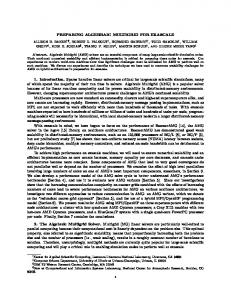
x

 π(

 k

 ) 

 

  
 
 
 
 
 
  


C  
 2i 
 
 
  





  
 
 
 
  






  
 
 
 
 
  

 
 
 
 x
 
 
  





     )  




 π( l
    




  
 
 
 
 
  



xi


















 

















x





 

























l



 












1 












C 



 























i 






































x



 










k


coarse grid point fine grid point

Figure 3.1. Point-symmetric grid at the fine grid point xi .

obtain

Aik

Aik cˆk

k∈Pi

´−1 ³ X

´³ X

Aik

´−1 ³ X

´ Aik cˆ

Aik

k∈Ni

´³ X

³ X

Aik

³ X

´ Aik cˆ

ˆC )i = −A−1 (IFDB Cc ii

³ X

=

−A−1 ii

=

−A−1 ii

k∈Ni

k∈Ni

k∈Pi

k∈Pi

k∈Pi

´

= c, for a fine grid point i ∈ F . Thus, constant functions are exactly interpolated independent of the underlying coarse grid. Note that this is in general not the case for the rotations. However, for some standard coarse grids, we can prove that also the rotations are reproduced exactly. To this end we define the notion of a point-symmetric grid. An example for a point-symmetric grid at a grid point xi in two dimensions is given in Figure 3.1. Definition 3.1. Let xi , i ∈ F , be a fine grid point. We call the grid Ωh := {xj | j ∈ N } point-symmetric at the grid point xi if there exist two disjoint subsets Ci1 , Ci2 ⊂ Ci , Ci1 ∪ Ci2 = Ci , a bijective function π : Ci1 7→ Ci2 and a constant vector c ∈ Rd so that the mapping Q(x) := −x + c is a bijection between supp(ϕli ) ∩ supp(ϕlk ) and supp(ϕli ) ∩ supp(ϕlπ(k) ) and Q(xk ) = xπ(k) for all k ∈ Ci1 . Theorem 3.2. Let xi , i ∈ F , be a fine grid point and let the grid Ωh be pointsymmetric at this point. Then, the rigid body modes, i.e. their coefficient vectors rˆ, are interpolated exactly at the point xi , (IF C rˆC )i = rˆi ∀ rigid body modes r.

(3.5)

Proof. It remains to prove the statement for a rotation r(x). Without loss of generality we assume that xi = 0. Since xi = 0 and therefore r(xi ) = 0, we have to 8

show (IF C rˆC )i = 0. For j ∈ Ci1 we have rˆj = −ˆ rπ(j) , so that ³ X

Aik

= −A−1 ii

³ X

= −A−1 ii

ˆC )i = −A−1 (IFDB Cr ii

´−1 X

´³ X

Aik

Aik

Aik

k∈Ci

´−1 X ³

Aik rˆk + Aiπ(k) rˆπ(k)

k∈Ni

´³ X

³ X

Aik

´³ X

Aik

´−1 X ³

Aik rˆk − Aiπ(k) rˆk

k∈Ni

k∈Ni

k∈Ci

Aik rˆk

k∈Ci

k∈Ci1

k∈Ci

k∈Ci1

´

´

holds. Therefore, it suffices to show that Aik = Aiπ(k) . Since ϕlk (x) = ϕlπ(k) (−x) is valid for all x ∈ supp(ϕlk ) ∩ supp(ϕli ), the application of the transformation rule of integration shows the equality (3.5). 4. Numerical Results. In this section we present the results of our numerical experiments with the block interpolation I B and point interpolation I P . We set the right hand side vector f to zero and start the iteration with a random valued initial guess u0 whose l2 -norm is equal to one, i.e. ||u0 ||l2 = 1. Due to this choice of parameters we have that the iterate uk (from the kth iteration) corresponds to the error ek = uk = uk − u. We stop the AMG-iteration when ||Auk ||l2 ≤ 10−12 and measure the speed of convergence by the asymptotic error reduction factor ¶1/10 µ ||uk ||l2 . (4.1) ρ := ||uk−10 ||l2 To give insight to the structure of the coarsening process and the coarser grids, we also give the total-grid-complexity, c(G) :=

J−1 X

niu /n0u ,

(4.2)

i=0

where niu denotes the number of grid points of the ith level, and J is the total number of the levels. The computational costs of one iteration step is important for the efficiency of the AMG method. Hence, we give an estimate of the computational costs associated with a single V-cycle via the total-operator-complexity, c(A) :=

J−1 X

niz /n0z ,

(4.3)

i=0

where niz is the number of nonzero blocks of the grid operator on the ith level. In all our experiments we set the parameter αtr for the truncation of the interpolation operator to 0.2 (compare subsection 3.2) and use the setup parameters α = 0.25 and β = 0.35 for the coarsening algorithm. Note that we coarsen down to a single grid point. We give numerical results for different discretized linear elasticity problems. First, we study the robustness of our point-block AMG with respect to the Poisson ratio ν and with respect to jumps of the elasticity modulus E for problems with vanishing Dirichlet boundary conditions. Then, we take a closer look at problems with free boundaries. Finally, we give results obtained for discretizations on complicated geometries and unstructured grids. 9

Table 4.1 Asymptotic error reduction ρ (4.1) and complexities c(A) (4.3) and c(G) (4.2) for Example 1 in two dimensions in the case of the point interpolation (PI) and the block interpolation (BI).

h 1/16 1/32 1/64 1/128 1/256

c(G) 1.72 1.69 1.68 1.68 1.67

PI c(A) 2.49 2.61 2.69 2.75 2.75

ρ 0.15 0.21 0.22 0.23 0.26

c(G) 1.73 1.70 1.68 1.67 1.67

BI c(A) 2.51 2.65 2.72 2.78 2.78

ρ 0.14 0.21 0.33 0.43 0.46

Table 4.2 Asymptotic error reduction ρ (4.1) and complexities c(A) (4.3) and c(G) (4.2) for Example 1 in three dimensions obtained with the point (PI) and block interpolation (BI).

h 1/16 1/24 1/32 1/40

c(G) 1.64 1.63 1.62 1.62

PI c(A) 3.25 3.38 3.44 3.48

ρ 0.18 0.23 0.27 0.28

c(G) 1.65 1.64 1.62 1.62

BI c(A) 3.64 3.87 3.97 4.02

ρ 0.16 0.21 0.26 0.29

Example 1 (h-stability and robustness with respect to the Poisson ratio). In the first example we study the independence of the rate of convergence ρ from the mesh-width for a discretization of (3.4) on the unit square/cube with Poisson ratio ν = 0.3 and Dirichlet boundary conditions. Table 4.1 shows the asymptotic error reduction rate ρ, the total-grid-complexity c(G) and the total-operator-complexity c(A) obtained for discretizations of the twodimensional problem for different mesh-widths h = 1/n. Both interpolations (the block interpolation and the point interpolation) lead to iterations which converge with a rate that is independent of the mesh-width. The point interpolation provides faster convergence than the block interpolation. For example, the asymptotic error reduction rate obtained with the point interpolation is ρ = 0.26 for h = 1/256 whereas we find ρ = 0.46 for the block interpolation. In three dimensions, both interpolations seem to give similar results. For a meshwidth of h = 1/40 we find ρ ≈ 0.3 which is comparable to the two-dimensional case. Note however, that the deterioration of the convergence rates for the block interpolation in two dimensions occurred for h ≤ 1/64 only. For h > 1/64 both interpolation schemes gave very much the same results. Hence, we may also find a deterioration of the block interpolation (asymptotically) in three dimensions. Note further that the operator-complexity c(A) = 4.02 obtained for the block interpolation (h = 1/40) is significantly higher in three dimensions than in two dimensions. This is an algorithmic problem and cannot be improved with the choice of a bigger truncation parameter αtr [16]. Another important property is the robustness of our point-block approach with respect to the Poisson ratio. The left picture of Figure 4.1 shows the asymptotic error reduction for the two-dimensional Dirichlet-problem on the unit square for a mesh-width h = 1/256 and different Poisson ratios ν. While the convergence results obtained for both interpolations are comparable for Poisson ratios less than 0.2, the point interpolation provides much better results for 0.2 < ν < 0.4 than the block interpolation. With the point interpolation out point-block AMG converges with an asymptotic error reduction rate of ρ = 0.23 whereas the block interpolation provides 10

0

1

10

PI BI

0.9

−2

0.8

10

0.7 −4

0.6

10

ρ 0.5

||e||

0.4

10

E

ν=0.0 ν=0.1 ν=0.2 ν=0.3 ν=0.34 ν=0.36 ν=0.4

−6

0.3 0.2

−8

10

0.1 0 0

0.1

0.2

ν

0.3

0.4

0

5

10

15

20

iter

Figure 4.1. Left: Asymptotic error reduction ρ (4.1) for Example 1 in two dimensions with h = 1/256 and varying Poisson ratios ν. Right: Convergence histories of a V(1,1)-cycle with the point interpolation and different Poisson ratios ν.

¾ h x2 ¾

6 h x1 - ? -

l Figure 4.2. Sketch of the mesh-structure used in Example 2 in two dimensions.

almost half the speed of convergence with ρ = 0.43 only. The point-block approach seems to be robust for Poisson ratios ν ≤ 0.36. The deterioration of the convergence rate ρ for Poisson ratios larger than 0.36 is not surprising and relates to the condition of the problem. As described in [1, Chapter 6] the condition of the elasticity problem depends on the Poisson ratio. The larger ν is, the worse the condition of the discretized problem is. This effect is also known as Poisson locking. Therefore, we fix the Poisson ratio at ν = 0.3 (which is a typical value in practice and smaller ν only improve the convergence results) for our remaining examples. Example 2 (The cantilever beam). In this example we focus on the problem of bad aspect ratios. We discretize the two-dimensional cantilever beam problem on a rectangular domain with the mesh width hx1 in the x1 -direction and hx2 = l · hx1 in the x2 -direction, where l > 0 is the stretching factor of the mesh as shown in Figure 4.2. In three dimensions we distinguish the two cases Ω = [0, l] × [0, 1]2 and hx1 = l · hx2 (= hx3 ), Ω = [0, l]2 × [0, 1] and hx1 = hx2 = l · hx3 ,

(4.4) (4.5)

as presented in Figure 4.3. In the two-dimensional case we expect similar results as for classical scalar AMG methods in the presence of anisotropic diffusion: Since the problem decouples more and more to a one-dimensional problem with a growing stretching factor l, AMG degenerates to a direct solver. Indeed, looking at Figure 4.4, where the convergence and complexity results for the two-dimensional problem with h = 1/256 are depicted, 11

Figure 4.3. The two different domains for the three-dimensional problem of Example 2. 1

3.5

PI BI

PI BI

3

0.8 c(A)

c(A)/c(G)

2.5 0.6

ρ

2 c(G)

1.5

0.4

1 0.2

0.5 0 1

2

4

8

l

16

32

64

128

0 1

2

4

8

l

16

32

64

128

Figure 4.4. Example 2 in two dimensions for h = 1/256 and the point (PI) and block interpolation (BI). Left: Asymptotic error reduction rate ρ (4.1) for different l. Right: Grid- (c(A) (4.3)) and operator-complexity (c(G) (4.2)).

we clearly see this expected behavior of our method. After a short decline of the speed of convergence for l ∈ [1, 4] for both interpolation operators, convergence speeds up. For l = 128 we obtain an asymptotic error reduction rate ρ = 0.06 for both interpolations. Furthermore, we find a decline of the total-operator-complexity c(A) for both interpolations when we increase l. For instance we have c(A) = 2.80 and c(G) = 1.65 for l = 1 and for l = 128 we find c(A) = 2.02 and c(G) = 2.06. This resembles the semi-coarsening of the method that can also be noticed for scalar anisotropic diffusion problems. In the three-dimensional case, we have to distinguish between the two different problem types (4.4) and (4.5). For the first problem (4.4), where the brick-type domain is only stretched in the x1 -direction, semi-coarsening appears only in one direction which does not influence the convergence rate ρ but the total-operator-complexity c(A). This fact becomes clear in Figure 4.5, which displays the results for h = 1/32. While the asymptotic error reduction rate ρ seems to be relatively independent of the parameter l, the total-operator-complexity is reduced from c(A) = 3.44 for l = 1 12

1

5

PI BI

4

c(A)

c(A)/c(G)

0.8

PI BI

0.6

3

ρ

0.4

2 c(G)

0.2

0 1

1

2

4

8

0 1

16

2

4

l

8

16

l

1

5

PI BI

0.8

PI BI

4

c(A)/c(G)

c(A)

0.6

3

ρ

0.4

2 c(G)

0.2

0 1

1

2

4

8

16

l

0 1

2

l

4

8

16

Figure 4.5. Example 2 in three dimensions for h = 1/32 and the point (PI) and block interpolation (BI). Upper left : Asymptotic error reduction ρ (4.1) for different l for problem type 4.4. Upper right: Grid- (c(A) (4.3)) and operator-complexity (c(G) (4.2)) for problem type 4.5. Lower left : Asymptotic error reduction ρ for different l for problem type 4.5. Lower right: Grid- (c(A)) and operator-complexity (c(G)) for problem type 4.5. Table 4.3 Convergence rates ρ (4.1) and complexity results c(A) (4.3) and c(G) (4.2) for Example 3 with h = 1/128 and the use of the point (PI) and block interpolation (BI).

E2 1 10 102 103 104

c(A) 2.75 2.81 2.81 2.80 2.80

PI c(G) 1.68 1.68 1.68 1.68 1.68

ρ 0.23 0.37 0.40 0.47 0.42

c(A) 2.78 2.86 2.85 2.84 2.84

BI c(G) 1.67 1.68 1.68 1.68 1.68

ρ 0.43 0.43 0.49 0.49 0.49

to c(A) = 2.57 for l = 16. The second problem (4.5) degenerates with growing l to a decoupled one-dimensional problem. Thus, the asymptotic error reduction rate and the total-operator-complexity decrease for growing l. Now, the method converges with ρ = 0.070 for l = 16 almost four times faster than in the case of l = 1 with ρ = 0.27. Example 3 (Jumps in the elasticity modulus). In practice, we are often confronted 13

Ω3

Ω4

Ω1

Ω2

1 2

1 2

Figure 4.6. The decomposition of the domain used in Example 3.

Figure 4.7. Hierarchy of grids generated for Example 3 of the method with point interpolation for h = 1/32 and E2 = 103 and h = 1/32 (larger points indicate coarser levels).

Table 4.4 Asymptotic error reduction rate ρ (4.1) for Example 4 with different numbers of free sides.

Number of free sides 0 1 2 3

1/64 0.32 0.53 0.69 0.83

BI 1/128 0.43 0.51 0.65 0.75

1/256 0.46 0.60 0.71 0.88

1/64 0.22 0.31 0.57 0.64

PI 1/128 0.23 0.30 0.49 0.69

1/256 0.26 0.28 0.54 0.70

with structural objects which are made of many different materials with different properties. This, however, leads to jumps in the coefficients of the elasticity operator, which makes the solution of the respective linear system even harder. In this example we examine such problems in two dimensions. Consider the decomposition of the domain Ω = [0, 1]2 into four sub-domains Ω1 , ..., Ω4 as shown in Figure 4.6. We set the Young modulus E to E1 = 1 in Ω1 and Ω4 , and to E2 = 10n in the other two sub-domains. Table 4.3 gives the convergence rates ρ and complexities c(A) and c(G) obtained for h = 1/128 and 0 ≤ n ≤ 4. As in the previous examples, the point interpolation provides better results than the block interpolation. But now the difference in the speed of convergence gets smaller for larger jumps of the elasticity modulus. While the convergence results of the block interpolation are almost constant, with the fastest convergence (ρ = 0.43) for n = 0 and the slowest convergence (ρ = 0.49) for n = 4, the convergence of our point-block AMG with the point interpolation decreases from ρ = 0.23 for n = 0 to ρ = 0.42 for n = 4. Although the convergence gets slower in comparison with the previous examples, it is still uniformly bounded with respect to the jumps of the elasticity modulus with ρ < 0.5 for both interpolations. The coarsening algorithm seems to detect the jumps in the elasticity modulus. This assertion is supported by the resulting hierarchy of grids shown in Figure 4.7 for h = 1/32 and n = 4. Example 4 (Free boundaries). In the previous examples homogeneous Dirichlet conditions were used on all boundaries. In practice, however, there are also Neumann boundary conditions or simply no conditions on some parts of the boundary. In this 14

Figure 4.8. Complete grid hierarchy (left) and first and second coarse grid (right) of Example 4 (h = 1/32) with three free sides (larger points indicate coarser level). Table 4.5 Asymptotic error reduction rate ρ (4.1) for Example 4 with a varying number of free sides and the different coarsening. PI denotes the point and BI for the block interpolation.

no separate coarsening separate coarsening of the complete boundary separate coarsening of the free boundary

1 0.30 0.27 0.24

h = 1/128 2 3 0.49 0.70 0.37 0.56 0.34 0.52

1 0.28 0.26 0.26

h = 1/256 2 3 0.54 0.70 0.34 0.59 0.30 0.54

example we therefore consider elasticity problems with free boundaries. The convergence deteriorates for a growing number of free boundaries, as we can see in Table 4.4 for the two-dimensional problem for h = 1/256 and a varying number of free sides. For example, our point-block AMG with the block interpolation I B converges in the case of three free sides and h = 1/256 with ρ = 0.70 three times slower than in the case of no free sides where we have ρ = 0.26. One reason for the increase in the convergence rates is the selection of points on the free boundary for the coarse grids. The complete coarse grid hierarchy and the first and second coarse grid for h = 1/32 and three free sides are shown in Figure 4.8. The coarse grid selection leads to a standard coarse grid for points in the interior but not for points lying on the boundary. Therefore, neither our block interpolation nor our point interpolation does reproduce the rigid body modes at such points exactly. Since this property is essential for the quality of our multilevel solver, the convergence deteriorates for a larger number of free sides. One way to overcome this problem is to develop a coarsening algorithm which provides a standard coarsening also for boundary points. Since the classic coarsening algorithm produces good results for interior points, it is natural to use this coarsening process in a first step to coarsen all boundary points separately and then, in a second step, to coarsen the interior points. To this end, it is necessary to separate the boundary grid points from the interior grid points. Since an AMG method should employ only algebraic information given through the stiffness matrix A, we have to develop a method which can find the boundary points purely with the help of algebraic information. Let us make the reasonable assumption supp(ϕqi ) ∩ supp(ϕqj ) 6= ∅ for any 1 ≤ q ≤ d ⇔ ∃1 ≤ k, l ≤ d : a(ϕki , ϕlj ) 6= 0. Then, it follows for regular rectangular grids that a point i belongs to the boundary, 15

1

1 dirichlet 1 free boundary 2 free boundaries 3 free boundaries

0.8

dirichlet 1 free boundary 2 free boundaries 3 free boundaries 4 free boundaries 5 free boundaries

0.8

ρ

0.6

ρ

0.6

0.4

0.4

0.2

0.2

0 1

1.1 1.2 1.3 1.4 1.5 1.6 1.7 1.8 1.9

ω

0 1

2

1.1 1.2 1.3 1.4 1.5 1.6 1.7 1.8 1.9

ω

2

Figure 4.9. Convergence results for Example 4 with the point interpolation. Left: Asymptotic error reduction rate ρ (4.1)in two dimensions, h = 1/256, in dependence of the relaxation parameter ω. Right: Asymptotic error reduction rate ρ in three dimensions with h = 1/16 plotted against the relaxation parameter ω using the point interpolation.

if it satisfies |Ni |