IEEE Transactions on Magnetics, Vol.34, No.5, Sept. 1998, pp. 3327-3330
An Algebraic Multigrid Method for Solving Very Large Electromagnetic Systems Ronny Mertens, Herbert De Gersem, Ronnie Belmans and Kay Hameyer Katholieke Universiteit Leuven, Dep. EE (ESAT), Div. ELEN, Kardinaal Mercierlaan 94, B-3001 Leuven, Belgium
Domenico Lahaye, Stefan Vandewalle and Dirk Roose Katholieke Universiteit Leuven, Dep. Computer Science, Celestijnenlaan 200A, B-3001 Leuven, Belgium Abstract — Although most finite element programs have quite effective iterative solvers such as an incomplete Cholesky (IC) or symmetric successive overrelaxation (SSOR) preconditioned conjugate gradient (CG) method, the solution time may still become unacceptably long for very large systems. Convergence and thus total solution time can be shortened by using better preconditioners such as geometric multigrid methods. Algebraic multigrid methods have the supplementary advantage that no geometric information is needed and can thus be used as black box equation solvers. In case of a finite element solution of a nonlinear magnetostatic problem, the algebraic multigrid method reduces the overall computation time by a factor of 6 compared to a SSOR-CG solver. Index terms — numerical analysis, electromagnetic analysis, iterative methods, finite element methods.
I. INTRODUCTION In finite element programs, direct methods are nowadays often replaced by iterative methods to solve the system of discretized linear equations. Stationary methods such as Jacobi, Gauss-Seidel and successive overrelaxation are straightforward to implement but usually not very effective. The conjugate gradient method, a non-stationary method, is harder to apply, but very effective when used in combination with a good preconditioner. Symmetric successive overrelaxation and incomplete Cholesky decomposition are often used as preconditioners for the CG method. Multigrid methods can be used as solvers. Their use as preconditioner often results in even more efficient iterative methods. II. MULTIGRID METHODS The concept of multigrid methods is not new. The basic idea of this iterative method is to combine computed results obtained on different scales, using results from one scale to wipe out certain error components of the approximation of the solution on another scale (Fig. 1 & 2). An extensive Manuscript received November 3, 1997. R. Mertens, +32 (0)16 321020, fax +32 (0)16 321985,
[email protected], http://www.esat.kuleuven.ac.be/ elen/elen.html; D. Lahaye, +32 (0) 16 327632, fax +32 (0)16 327996,
[email protected], http://www.cs.kuleuven.ac.be/ cwis/dept-E.html. The authors are grateful to the Belgian "Fonds voor Wetenschappelijk Onderzoek Vlaanderen" for its financial support of this work and the Belgian Ministry of Scientific Research for granting the IUAP No. P4/20 on Coupled Problems in Electromagnetic Systems. The research Council of the K.U.Leuven supports the basic numerical research.
13
Fig. 1. Error after 0, 2 and 50 Jacobi iterations.
Fig. 2. Error after 2 Jacobi iterations projected on a coarser grid.
treatment of multigrid methods can be found in [1]-[3]. Here, the main ideas are briefly recalled. The finite element discretization on a mesh of size h, of a diffusion problem, e.g. Poisson's equation, leads to a system of linear equations of the form
A h xh = bh ,
(1)
where A h is a sparse, symmetric and positive definite matrix, b h the right-hand side vector and x h the solution vector. Stationary iterative solvers have a general form of
(
)
x hk +1 = x hk − M h−1 A h x hk − b h ,
(2)
e.g. Jacobi ( M h is the diagonal of A h ) or Gauss-Seidel ( M h is the lower triangular part of A h ). The error x h − x hk can be seen in the Fourier space as a linear combination of
IEEE Transactions on Magnetics, Vol.34, No.5, Sept. 1998, pp. 3327-3330
sinusoidal waves. Certain classes of stationary methods, so-called smoothers, effectively reduce the short waves (high frequency components) in the error (Fig. 1). Convergence stalls, however, as soon as the error becomes smooth. Slowly varying functions, such as the smoothed error, can be represented on coarser meshes without too much loss of information (Fig. 2). Because these functions are seen on a larger scale, they appear to be more oscillatory again. The idea in multigrid is to use a hierarchy of continuously coarser grids and to exploit the smoothers to filter out the high frequency error components on each grid. One iteration of a basic two-grid iterative process consists of different steps (Fig. 3). A few (for example two) error smoothing steps are applied on the fine grid. xhk is the obtained approximation of the solution after smoothing. The defect
dhk = b h − A h xhk
(3)
is projected onto a coarser grid with mesh size H, where a coarse grid correction term is computed. This projection is denoted by d kH . The coarse grid correction e kH is the solution of
A H e kH = d kH
(4)
with A H the coarse grid equivalent of A h . As the coarse grid contains less points than the original fine grid, solving (4) is substantially cheaper than solving (1). The correction term is interpolated on the fine grid, which gives added to the previous approximation.
xhk = xhk + e hk
e kh ,
and
(5)
Finally, as the latter operation reintroduces high frequency error components to the existing approximation, a few postsmoothing steps have to be performed. In the multigrid extension of the two-grid method the latter is recursively called, to compute the coarse grid correction until the coarseness of the mesh makes the cost of applying a direct solver negligible. As the multigrid method is a stationary iterative process, its iterates can also be cast into the form (2) for some matrix M h . Unlike the previously mentioned solution methods, the number of iterations required by multigrid techniques in order to obtain a prescribed accuracy is independent of the mesh size. In this sense multigrid methods are optimal [1],[4]. In computing the solution by using a multigrid technique, not only the matrix and right-hand side are required, but a sequence of coarser grids as well. This makes the implementation of a multigrid technique more involved than that of a single grid iterative method.
x hk
apply presmoothing
add correction
project on coarse grid
interpolate on fine grid
apply postsmoothing
x hk +1
compute coarse grid correction
Fig. 3. Scheme of a two-grid method.
III. ALGEBRAIC MULTIGRID METHODS A. Algebraic Multigrid Method as Solver The algebraic multigrid method (AMG) imitates a geometric multigrid method by using information about the system matrix only. This makes AMG attractive as black box solver. In AMG a set-up phase and a cycling phase are distinguished. A hierarchy of coarser grids is automatically generated in the set-up phase. The coarse grid is seen as a subset of the fine grid. The points i and j are called strongly connected to each other if the matrix entry A ij is large enough. The points of the coarse grid are chosen in such a way that [5]: • each point in the coarse grid is strongly coupled to at least one point in the fine grid, • and no two points in the coarse grid should be strongly connected to each other. Once the sequence of grids, projection and interpolation operators are defined, the iteration process proceeds similar to a geometric multigrid. B. Algebraic Multigrid Accelerated by Outer CG Iteration Stationary methods of type (2) can often be accelerated by conjugate gradient or, more generally, Krylov subspace methods [6]. The stationary method is then called a preconditioner of the accelerated scheme. If a linear method is only slowly convergent, or even divergent, it may still make a very effective preconditioner. The lack of satisfactory convergence of the unaccelerated method is often due to the particular nature of the spectrum of M h−1A h . This may consist of clusters of points surrounded by a few outlyers, the latter being the cause of the slowdown or divergence. The CG or Krylov method removes the error components associated with the outlyers very effectively. Hence these methods notably accelerate the linear method, they also make the overall iteration more robust. This is achieved at a fairly
14
IEEE Transactions on Magnetics, Vol.34, No.5, Sept. 1998, pp. 3327-3330
0.2
0
-0.2 0
0.2
0.4
0.6 Eigenvalues
0.8
1
1.2
Fig. 4. Spectrum of the matrix M h−1 A h .
negligible cost. Fig. 4 gives the spectrum of M h−1A h for one of the calculations of the example. C. Implementing the Acceleration
Fig. 5. Initial (1092 nodes) and intermediate mesh (11147 nodes) of a synchronous line-start motor.
The implementation of a preconditioner for CG involves the computation of
z = M −h 1 r
(6)
as one of the steps in the algorithm. r and z are the residual and the new search direction respectively and M h is the matrix that identifies the particular preconditioner. By comparing (2) and (6), it can be seen that AMG can be implemented as preconditioner without explicit knowledge of the M h matrix. Therefore, the right-hand side in (2) is set to be equal to the residual, the starting solution equal to zero, and one iteration of AMG is computed. IV. COMPARISON OF THE DIFFERENT SOLVERS
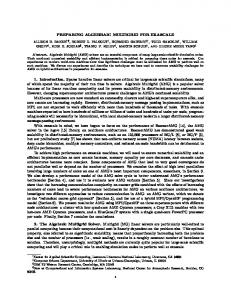
Fig. 6. Field plot of a synchronous line-start motor (11147 nodes). 2:30:00 IC-CG 2:00:00 Total solution time
To compare the total solution time of different solvers, a synchronous line-start motor excited with permanent magnets is taken as an example. Saturation plays an important role in the behaviour of this machine. Fig. 5 shows the initial and an intermediate mesh of the finite element model. The field plot of the corresponding intermediate solution is shown in Fig. 6. Values of the nodal flux densities weighted with the energy in an element are used as an a posteriori error estimator. 13 adaptation steps were calculated on a HP C-160 workstation. Fig. 7 shows the total solution times after each adaptation step for the different methods. The AMG code is implemented by [5]. AMG accelerated by an outer CG iteration is 40% faster than AMG used as solver. Fig. 8 shows the average number of iterations per Newton step in each adaptation step. The linear system in each Newton step
SSOR-CG AMG AMG-CG
1:30:00
1:00:00
0:30:00
0:00:00 1.0E+03
1.0E+04 1.0E+05 Number of nodes
Fig. 7. Total solution times after each adaptation step.
15
1.0E+06
IEEE Transactions on Magnetics, Vol.34, No.5, Sept. 1998, pp. 3327-3330
V. CONCLUSION
80 AMG Average number of iterations
AMG-CG
60
40
20
0 0
1
2
3
4 5 6 7 8 9 Number of adaptation step
10
11
12
13
Fig. 8. Average number of iterations per Newton step.
Despite the extra cost per iteration by applying an algebraic multigrid method as preconditioner for the conjugate gradient method (AMG-CG), the solution time is reduced by a factor of 2 for small problems and a factor of 6 for very large problems, when compared to symmetric successive overrelaxation as preconditioner (SSOR-CG). The increase to 180 % (82.5 MB instead of 45.5 MB for 243620 nodes for a non-linear problem) in allocated memory for storing and solving the system of linear equations, is therefore worth paying. As AMG can be used as a black box solver, AMGCG promises to be very well suited to solve 3D problems where the solution time increases even more rapidly and the geometric construction of coarse meshes is even more troublesome than in the 2D case. REFERENCES
is iterated to convergence (machine precision). The number of iterations is practically independent of the number of nodes. To solve the system after 13 adaptation steps (243620 unknowns), AMG-CG required only an average of 18 CG iterations in the last Newton step, while AMG needed 47 cycles.
[1] W. Briggs, A Multigrid Tutorial, SIAM, Philadelphia, 1987. [2] W. Hackbusch, Multi-Grid Methods and Applications, Springer-Verlag, Berlin, 1985. [3] C.C. Douglas, “Multigrid methods in science and engineering,” IEEE Computational Science and Engineering, 1996, pp. 55-68. [4] G. Golub and C. Van Loan, Matrix Computations, The Johns Hopkins University Press, 1989. [5] J. Ruge and K. Stueben, Multigrid Methods, SIAM, Philadelphia, 1987. [6] Y. Saad, Iterative Methods for Sparse Linear Systems, PWS Publishing Company, Boston, 1996. [7] R. Barrett et al., Templates for the Solution of Linear Systems: Building Blocks for Iterative Methods, SIAM, Philadelphia, 1994.
16