An Algorithm and Hardware Architecture for Integrated Modular Division and Multiplication in GF (p) and GF (2n ) Lo’ai A. Tawalbeh and Alexandre F. Tenca School of Electrical Engineering and Computer Science, Oregon State University, USA email: tawalbeh,
[email protected] Abstract This paper presents an algorithm and architecture that integrates modular division and multiplication in both GF (p) and GF (2n ) fields (Unified). The algorithm is based on the Extended Binary GCD algorithm for modular division and on the Montgomery’s method for modular multiplication. For the division operation, the proposed algorithm uses a counter to keep track of the difference between two field elements and this way eliminate the need for comparisons which are usually expensive and time-consuming. The proposed architecture efficiently supports all the operations in the algorithm and uses carry-save unified adders for reduced critical path delay, making the proposed architecture faster than other previously proposed designs. Experimental results using synthesis for AMI 0.5µm CMOS technology are shown and compared with other dividers and multipliers.
1.
Introduction
Given the increasing demand for secure communications, cryptographic algorithms will be embedded in almost every application involving exchange of information. Modular arithmetic operations such as division and multiplication over finite fields (mostly GF (p) and GF (2n )), are widely used in several cryptographic applications. In general, public-key cryptographic algorithms requires a huge amount of computations, therefore, there is an increasing demand for dedicated hardware to accelerate these computations. An algorithm and hardware implementation that is able to compute modular division and multiplication in both GF (p) and GF (2n ) is definitely advantageous. The modular multiplication operation with a large modulus is very important in many public-key cryptosystems. Montgomery multiplication algorithm [11] is an efficient way to compute modular multiplication. Authors in [5] proposed a unified algorithm to compute Montgomery multiplication in both GF (p) and GF (2n ). On the other hand, modular division and modular inverse are time consuming operations and they cannot be avoided completely in practical applications. For instance, they are used in decryption of ElGamal [7] public-key cryptosystem. Researchers have claimed that a gain in performance can be obtained when they are implemented in hardware [1, 6]. The Unified modular Division/Multiplication Algorithm (UDMA) proposed in this work computes modular division and Montgomery multiplication in both GF (p) and GF (2n ) fields. The UDMA is based on the Extended Binary GCD algorithm [2, 12] for
modular division and on the Montgomery’s method for modular multiplication. For the division operation, the proposed algorithm uses a counter to keep track of the difference between integers in GF (p) or polynomial degrees in GF (2n ), reducing the complexity of each algorithm iteration by eliminating the need for comparisons of field elements. Other modular division (inverse) algorithms have integer and polynomial degree comparisons [6, 8, 9] as part of their control flow. The hardware architecture for the unified divider/multiplier that implements the UDMA efficiently supports all the computations in the algorithm and uses Carry Save representation so that all additions and subtractions are done in constant time, independent of the operands precision. The following Section presents some general concepts and mathematical notation used in this paper. The Unified modular Division/Multiplication Algorithm (UDMA) is proposed in Section 3. The overall organization of the hardware design that implements the UDMA and its main functional blocks are shown and described in detail in Section 4. Experimental results are shown in Section 5, followed by conclusions in Section 6.
2.
General Concepts and Notation
The element Y (x) ∈ GF (2n ) is a polynomial of degree less than n and has coefficients in GF (2). In this paper, we consider polynomial basis for the elements of GF (2n ). On the other hand, the element Y ∈ GF (p) is an integer in the set {1,..., p − 1}, where p is a n-bit prime modulus in the range 2n−1 < p < 2n . Elements in both fields are represented as bit vectors. For simplicity Y (x) is denoted as Y in the algorithm description. The addition in GF (2n ) is a polynomial addition, which is done as a bitwise logic exclusive OR operation between the two bit vectors being added. An irreducible polynomial p(x) of degree n is used to reduce intermediate results in GF (2n ). On the other hand, the addition of elements in a prime field is a conventional integer addition with modulo reduction (mod p). • Extended Binary GCD Algorithm for Modular Division in GF (p) and GF (2n ): Extended Binary GCD algorithm is an efficient way to compute modular division (inversion) [2, 12, 10]. A unified division algorithm based on the Extended Binary GCD algorithm was presented in [2]. The algorithm computes the modular division in either GF (p) or GF (2n ) fields for inputs X, Y, p and F ield. The computation Z = X Y mod p is performed X(x) when F ield = GF (p), and Z(x) = Y (x) mod p(x) is done when F ield = GF (2n ). In both cases, Y 6= 0. The modular inverse can be obtained by forcing X = 1. Notice that the division or inverse takes the same amount of time. • Unified Montgomery Modular Multiplication Algorithm: Montgomery introduced an efficient algorithm to calculate modular multiplication [11]. A Montgomery algorithm to handle multiplication in GF (p) and GF (2n ) finite fields was introduced in [5]. The Montgomery multiplication algorithm generates the product of two n-bit integers X and Y in modulo p as: M M (X, Y ) = XY r−1 mod p, where r = 2n for 2n−1 < p < 2n . The modulus p and the constant r must be relatively prime. This condition is easily satisfied when p is odd. The Montgomery image of an integer a, represented as a ¯, can be obtained by multiplying it by the constant r and reducing it modulo p: a ¯ = ar mod p.
3.
Unified Algorithm for Modular Division and Montgomery Modular Multiplication. The Unified modular Division/Multiplication Algorithm (UDMA) is stated as follows:
Function: Modular Division and Multiplication in GF (p) and GF (2n ) Inputs: 0 ≤ X < p, 0 < Y < p, 2n−1 < p < 2n , F ield, Op, n Output: Z = XY 2−n mod p when Op = mult, Z = X mod p when Op = div. Y Algorithm: C =Y. IF Op = mult THEN /* M ultiplication M ode */ D = 0, U = 0, W = X, δ = n ELSE /* Division M ode */ D = p, U = X, W = 0, δ = 0 END IF; WHILE [(C 6= 0 AND Op = div) OR ( δ 6= 0 AND Op = mult)] IF c0 = 0 THEN C := C À 1 δ := δ − 1 /* Integer Operation */ ELSE k=1 IF (Op = div) THEN IF δ < 0 THEN C ⇔ D, U ⇔ W , δ := −δ END IF; /* Swapping */ IF((C + D) mod 4 6= 0 AND F ield = GF (p)) THEN k = −1 ELSE δ := δ − 1 END IF; ELSE /* Op = mult */ δ := δ − 1 END IF; C := (C + k ∗ D) À 1, U := (U + k ∗ W ) END IF; U := (U + u0 ∗ p) À 1 END WHILE; IF Op = div THEN Z := W ELSE Z := U END IF;
To the best of our knowledge, this is the first algorithm that integrates the computation of modular division and Montgomery modular multiplication in both GF (p) and GF (2n ). The UDMA mode of operation is controlled by input Op (div or mult), and the finite field is controlled by the input F ield (GF (p) or GF (2n )). For simplicity, the polynomials X(x), Y (x), and p(x) are denoted as X, Y , and p, respectively, which correspond to the bit-vector representation of these polynomials. Most of the arithmetic operations in the algorithm are common to both modes of operation. The initialization of variables depends on the operation. For a given field, all the additions/subtractions are done in the field, besides the arithmetic operations on δ (subtractions and change of sign) which are always integer operations. The algorithm integrates the Extended Binary GCD algorithm and the Montgomery multiplication algorithm and it was verified using Maple. To compute Montgomery multiplication using an n-bit modulus p, UDMA performs n iterations. The counter δ is initialized with value n, and in each iteration it is decremented by one. The variables used in the algorithm are initialized as: C = Y , D = 0, U = 0, and W = X. The result is ready (Z = U ) when δ = 0. The partial product U is reduced mod p in each iteration. In both fields, while multiplying, addition is used in the operations that update C and D (k = 1). The À operator indicates a 1-bit right shift operation.
The UDMA computes modular division using the same structure used by the Extended Binary GCD Algorithm for modular division [2]. The variables are initialized as: C = Y , D = p, U = X, W = 0, and δ = 0. If the division is computed in GF (p), UDMA tests the least significant two bits of C and D ((C + D) mod 4 6= 0) to conditionally subtracts C from D (set k = −1). Otherwise, C is always added to D in both fields. The division is completed when C = 0, and the final result is available in W . More details about the operation of the UDMA are presented in the following Section.
4.
Overall Hardware System Architecture
Figure 1 shows the top level architecture of the Unified Modular Divider/Multiplier (call it UMDM) that implements the UDMA. The main functional blocks are Register File (RF), Datapath, and Control. More details about these blocks are provided next. Op Field n
Control 3
n input (X,Y,P)
2 vectors
3
3
in dst src1 src2
2n Load
Y
out1
(2 vectors) 2n
A
UMDM Datapath
Register File (RF) out2
(2 vectors) 2n
B Sum / Carry (2 vectors) 2n
Load
Figure 1. Top level hardware architecture of the unified modular divider/multiplier (UMDM). 4.1.
Register File
The register file has five registers (R1 to R5). Since the computations are done in Carry-Save form, each intermediate variable (C, U, D, W ) is represented in two vectors (sum,carry). So, the registers inside the register file are designed to store two n-bit vectors. In other words, the ith register Ri is represented as Ri = (sum, carry) = (Ri s, Ri c). The register file has one input, and two output ports. The Control block provides the register file with the signals necessary to perform reading/writing operations. The 3-bit signal dst determines the destination register to be written. The signals src1, src2 (3-bits each), specify the registers to be read at output ports out1, out2, respectively. 4.2.
UDMA Datapath
The n-bit datapath implementing the UDMA is shown in Figure 2. Each “while iteration” of the algorithm is implemented in 1 clock cycle for multiplication mode, and
in 3 clock cycles for division if C is odd, and 2 clock cycles if C is even, as explained later. As
Ac
Bs
a
b
c
Bc N
FSEL
Unified Carry-Save Adder1 with Complement (UCSA1)
complementer
NEG C in
sel_zero
LSBit of U (u0 )
Y LoadY shiftY
Yshifter (c 0)
AND FSEL
C
Unified Carry-Save Adder2 (UCSA2)
in
control
result_shifter Sum
sh
shift
Carry
Figure 2. Unified datapath of the modular divider/multiplier (UMDM datapath). The proposed datapath has two inputs represented in carry-save form as A=(As,Ac) and B=(Bs,Bc) which receive their values from the register file ports (out1, out2), respectively. The main components of the datapath are two (3-2) Unified Carry-Save Adders (UCSAs) which are similar in complexity to full-adders [5]. The unified adders can perform bit addition with or without carry depending on the input FSEL (Field Select). The unified adder may be used to implement a redundant or non-redundant adder.The use of non-redundant form of the operands and results reduces the register area but increases the addition time (because of carry propagation).We decided to use Carry Save adders to make the addition time constant and independent of the operand’s precision. 4.2.1. Unified Carry-Save Adders: The first adder in the datapath is a Unified Carry-Save Adder with complement (UCSA1). Figure 4.a shows the bit slice diagram for this adder and Figure 4.b shows the connection of n slices to form an n-bit adder. The UCSA1 outputs are: (sum, carry) = a+b+c when N EG = Cin = 0, and (sum, carry) = a + b − c when N EG = Cin = 1. Addition and subtraction in GF (2n ) are the same. NEG c
an-1 bn-1 cn-1 FSEL
a1 b1 c1
a0
b0 c0
FSEL
FSEL
sum
b a
NEG
FSEL
UCSA1
UCSA1
UCSA1
1-bit
1-bit
1-bit
carry C in carry n
(a) bit slice
sum n-1 carry n-1
sum 1 carry 1
sum 0 carry 0
(b) n-bit adder
Figure 3. Unified carry-save adder with complement (UCSA1) for 1-bit and n-bit precision.
As we can see from Figure 3, the change of sign operation inside the UCSA1 is done in parallel with the addition operation, and so, it does not add to the critical path. The AND gate shown at the top of UCSA2 in Figure 2 is used to select between the value 0 or the modulus p depending wether U is even or odd (this is determined by testing u0 ), respectively. The input signal sel zero when asserted forces the third input of the UCSA2 to zero. The delay of the UMDM datapath (tdatapath ) is determined by the delay of the two UCSAs, the delay of the AN D gate between them, and the delay of the result shif ter which has a delay of 2-input multiplexer (tM U X ' tXOR ). By integrating the AND gate with the second adder (shown in dashed box in Figure 2), its delay will not add to the path delay. Knowing that each UCSA has a delay of a full adder (tF A = 2tXOR ), we get: tdatapath = tU SCA1 + tU CSA2 + tresult
shif ter
= 4tXOR + tM U X = 5tXOR
The Yshifter shown in Figure 2 is a shift register used to implement the operation (C >> 1) only in the multiplication mode. It is loaded with the input Y (multiplier) when laodY = 1. When shif tY = 1, C is shifted right by 1-bit (remember that C = Y ). The least significant bit of the shifted C goes to the control section to be tested (c0 = 0). The datapath outputs (Sum, Carry) are shifted right 1-bit by correct wiring using the result shif ter at the output of the UCSA2. This module is implemented as two 2-input multiplexers with select line shif t. When shif t = 1, the shifted outputs are selected. 4.3.
Control Block
This section describes the Control block and the system operation during division and multiplication modes and the design techniques used to implement the proposed UMDM. When Load = 1, the registers inside the register file are initialized (by the user) with the inputs X,Y , and p depending on the operation to be performed by the algorithm. While the algorithm is in division mode, the test C 6= 0 must be done. The vector C is in Carry Save form. Simulation results show that C = 4 or −4 at the end of computation. If more iterations than required are performed, the result is still correct. In the proposed UMDM design, the test C 6= 0 is replaced by testing the bit vector C for specific values (4 or -4), and no need to compare all the bits of C with zero. 4.3.1. Multiplication Mode: The proposed multiplier/divider performs 1 iteration of the algorithm in each clock cycle when computing Montgomery multiplication in both fields. Only three registers are used. Table 1 shows the loading phase for multiplication and division (initialization of the intermediate variables) as described by the algorithm. Table 2 shows the operation of the unified divider/mulitplier when performing Montgomery multiplication in GF (p) or GF (2n ). It shows the main control signals applied to the register file and the datapath to compute multiplication. The values of the signals which are not mentioned in the Table are equal to zero. Depending on C (even or odd), a different set of signals are used. The Table also shows the interpretation of these signals on the datapath, and the corresponding operation in the UDMA. When c0 = 1, two additions (U := (U + k ∗ W ) and U := (U + u0 ∗ p) >> 1) are performed by the datapath. The variable C is shifted right one bit using the Y shif ter in every cycle (shif tY ← 1). The counter δ is initialized with n to indicate the number of iterations. Since δ is decre-
Table 1. Load phase for multiplication and division
Multiplication Variables/parameters Loading the RF represented by R R ← (Rs, Rc) W and p R1 ← (X, p) U R2 ← (0, 0) p R3 ← (0, p) Variable Loading the Shifter C YShifter ← (Y )
Division Variables/parameters Loading the RF represented by R R ← (Rs, Rc) W R1 ← (X, 0) U R2 ← (0, 0) D R3 ← (p, 0) C R4 ← (Y, 0) p R5 ← (0, p)
Table 2. The operation of the UMDM during Montgomery multiplication c0 = 0 (then) Control Datapath Signals Interpretation src1 ← (010) (As, Ac) ← (U s, U c) src2 ← (011) (Bs, Bc) ← (0, p) dst ← (010) store the result in U shif tY ← 1 C >> 1 shif t ← 1 the result >> 1 dec delta ← 1 δ = δ − 1 Computes: U := (U + u0 ∗ p) >> 1
c0 = 1 (else) Control Datapath Signals Interpretation src1 ← (010) (As, Ac) ← (U s, U c) src2 ← (001) (Bs, Bc) ← (X, p) dst ← (010) store the result in U shif tY ← 1 C >> 1 shif t ← 1 the result >> 1 dec delta ← 1 δ = δ − 1 U := (U + k ∗ W ), U := (U + u0 ∗ p) >> 1
mented by one in each iteration (dec delta = 1), the computation ends when δ = 0, and the result can be read form R2 . 4.3.2. Division Mode: Each modular division iteration in the proposed UMDM architecture requires 2 clock cycles if C is even and 3 clock cycles if C is odd in both fields. The initialization of variables was shown in Table 1. Let us assume that the algorithm is computing modular division in GF (p). Tables 3 and 4 show the control signals during division when C is even and odd, respectively. Table 3 shows when δ is positive, the expression U := (U + u0 ∗ p) >> 1 is computed in the first clock cycle. C is shifted right by 1-bit (C >> 1) in the second cycle in order to enable the test for c0 = 0 which decides on the control signals of the next iteration.
Table 3. The UMDM operation during computing division when c0 = 0 Clock Cycle cycle 1
cycle 2
c0 = 0 (then) State1: Original State2: Swapped Control Datapath Control Datapath Signals Interpretation Signals Interpretation src1 ← (001) (As, Ac) ← (U s, U c) src1 ← (010) (As, Ac) ← (W s, W c) src2 ← (101) (Bs, Bc) ← (0, p) src2 ← (101) (Bs, Bc) ← (0, p) dst ← (001) store result in R1 (U ) dst ← (010) store result in R2 (W ) shif t ← 1 result >> 1 shif t ← 1 result >> 1 U := (U + u0 ∗ p) >> 1 is computed src1 ← (100) (As, Ac) ← (Cs, Cc) src1 ← (011) (As, Ac) ← (Ds, Dc) sel zero ← 1 (Bs, Bc) ← (0, 0) sel zero ← 1 (Bs, Bc) ← (0, 0) dst ← (100) store result in R4 (C) dst ← (011) store result in R3 (D) shif t ← 1 result >> 1 shif t ← 1 result >> 1 dec delta ← 1 δ = δ − 1 dec delta ← 1 δ = δ − 1 C := (C) >> 1 is computed
Table 4. The UMDM operation during division when c0 = 1 Clock Cycle cycle 1
cycle 2
cycle 3
c0 = 1 (else) State1: Original State2: Swapped Control Datapath Control Datapath Signals Interpretation Signals Interpretation src1 ← (001) (As, Ac) ← (U s, U c) src1 ← (010) (As, Ac) ← (W s, W c) src2 ← (010) (Bs, Bc) ← (W s, W c) src2 ← (001) (Bs, Bc) ← (U s, U c) dst ← (001) store result in R1 (U ) dst ← (010) store result in R2 (W ) shif t ← 0 result is not shifted shif t ← 0 result is not shifted dec delta ← ∗, *=1 when T EST = 0, otherwise *=0. (δ = δ − 1) U := (U + k ∗ W ) is computed src1 ← (001) (As, Ac) ← (U s, U c) src1 ← (010) (As, Ac) ← (W s, W c) src2 ← (101) (Bs, Bc) ← (0, p) src2 ← (101) (Bs, Bc) ← (0, p) dst ← (001) store result in R1 (U ) dst ← (010) store result in R2 (W ) shif t ← 1 result >> 1 shif t ← 1 result >> 1 negate delta ← ∗, *=1 when δ < 0, otherwise *=0. (δ = −δ) U := (U + u0 ∗ p) >> 1 is computed src1 ← (100) (As, Ac) ← (Cs, Cc) src1 ← (011) (As, Ac) ← (Ds, Dc) src2 ← (011) (Bs, Bc) ← (Ds, Dc) src2 ← (100) (Bs, Bc) ← (Cs, Cc) dst ← (100) store result in R4 (C) dst ← (011) store result in R3 (D) shif t ← 1 result >> 1 shif t ← 1 result >> 1 C := (C + k ∗ D) >> 1 is computed
The Control during division has two major ”states”: Original (not swapped) and Swapped. The control goes back and forth between these states only when c0 = 1 and δ < 0. The sign of δ is made positive (δ = −δ) when this condition happens (realized by the control signal negate delta as shown in Table 4). When the control state is Original, the variables W, U, D, C are read from the registers R1 , R2 , R3 , R4 , respectively. Also, the updated values of these variables are written to the above registers in the same order. When the control state is Swapped, the sources for the variables W and U are reversed (W is read from R2 and U from R1 ). Same thing applies for C and D (C is read from R3 and D from R4 ). The same approach is used for writing to these variables. This way, the swap operation is realized by reading from/writing to the correct register. The value of k ∈ {-1,1} is determined by the control section depending on the result of the test ((C + D) mod 4 = 6 0 AN D F ield = GF (p)), which is denoted by (T EST ) in Table 4. In the case k = −1, negative D and negative W are obtained by setting N = 1. Since the T EST is done on the least two significant bits of C and D, it can be implemented using a two-level gate network. If the algorithm is computing the modular division in GF (2n ), the same procedure described above is followed, except that the T EST is not applicable (F ield = GF (2n )). For both fields, the computation is completed when C = 0, and the result is Z = W .
5.
Experimental Results and Comparisons
This section has two categories of experimental results: (a) number of iterations obtained from a Maple model and (b) the critical path delay results obtained by synthesis of the VHDL description of the algorithm.
5.1.
The Number of Iterations
Maple was used to describe the proposed algorithm (Alg1 = U DM A) and the unified Montgomery inverse algorithm presented in [6] (Alg2). At least 100 random samples were used to verify each algorithm operation and obtain statistics. The other division (inversion) algorithm being compared is the unified Montgomery inverse algorithm presented in [6] (Alg2). For consistency, no multiple-word calculation is considered here. For an n−bit input Y , Alg2 computes Z = Y −1 2k , where n ≤ k ≤ 2n is the number of algorithm iterations. A correction step is needed to get the inverse in the Montgomery domain (Y −1 2n ) or in the integer domain (Y −1 ). Therefore, the total number of iterations required to compute the inverse in Montgomery domain is 2k − n. To compute the modular inverse in the integer domain it needs 2k iterations. Number comparisons were used in Alg2 to compare the size of the bit vectors that represent elements in the field (the same way it was done in [1, 8, 9]) instead of the counter (δ) used in our algorithm. The comparison limits a fast hardware implementation. Figure 4 shows the number of iterations as a function of operand size required by Alg1 (UDMA) and Alg2 to compute the integer modular inverse (division) in GF (p) and GF (2n ). The size of the operands is in the range (160 to 512) bits. From figure 4, we can see that Alg1 executes in about 25% less iterations than Alg2 when computing the inverse in the integer domain for GF (p). For GF (2n ), Alg1 has about 40% less iterations than Alg2 when computing the inverse in the integer domain. Notice that the number of iterations for Alg1 in both fields increase linearly with the operand precision. 1800 1600
Iterations
1400 1200 1000 800
Alg1 GF(p) Alg2 GF(p) Alg1 GF(2^n) Alg2 GF(2^n)
600 400 200 0 0
100
200
300
400
500
600
Operand size (bits)
Figure 4. The number of iterations as a function of operand size required by Alg1 (UDMA) and Alg2 (presented in [6]) to compute the modular inverse in GF (p) and
GF (2n ) J. Goodman et al. presented in [8] a public-key processor that implements operations required for Elliptic Curve Cryptography (ECC) including modular inverse in GF (2n ) only. It is stated in [8] that the inversion in GF (2n ) takes on average 3.3 cycles for each bit. Alg1 needs a maximum of 2 iterations/bit and on average 1.5 iterations/bit to compute the modular inverse in GF (2n ). The UMDM architecture performs each iteration of Alg1 in 2.5 clock cycles on average. Therefore, the GF (2n ) inversion by Alg1 takes on average 1.5 × 2.5 = 3.75 cycles for each bit. But on the other hand, the critical path delay (clock period) of the datapath of the processor presented in [8] (call it tGµP ) is the delay of 2 full adders (tF A ) and 2 levels of muxes and an AN D gate
(tGµP = 2tF A + 2tmux + tAN D ), compared to a critical path delay of only 2 full adders and 1 level of muxes for the UMDM datapath proposed in this work (tU M DM = 2tF A + tmux ). The critical path delay will affect the total computational time as will be seen later. Alg1 computes Montgomery modular multiplication in n cycles, which is consistent with several other designs [5, 8, 11]. 5.2.
Synthesis Results
The experimental data presented in this section were generated using Mentor Graphics CAD tools. The target technology was set to AM I05 f ast auto (0.5 µm CMOS with hierarchy preserved) provided in the ASIC Design Kit from the same company[3]. The UMDM architecture was described in VHDL and simulated in ModelSim for functional correctness. It was synthesized using Leonardo tool for the mentioned technology. Figure 5 shows the critical path delays (in nano-seconds) of the UMDM for the precision range (160-512) bits. The Figure shows that the delay increases with the number of bits and it saturates at higher precision. This indicates that the critical path delay (clock period) of the UMDM became independent of the operands size at high precisions.
Time (nano seconds)
13
12 0
100
200
300
400
500
600
Operand size (bits)
Figure 5. The critical path delay of the UMDM in nano-seconds (operand size from 160-512 bits). The public-key processor presented in [8] (GµP ) runs at clock rate of 50 MHz (clock period = 20 nsec), and it is considered a good representative of this class of hardware designs. The divider/multiplier proposed in this work has a maximum clock period of 12.8 nsec at 512-bit operand size, which is about 1.6 times faster than GµP . Also, as mentioned before, the GµP takes 3.3 cycles/bit to perform a modular inverse in GF (2n ) and this design takes 3.75 cycles/bit. Let the total average computation time of a given design Tdesign : Tdesign = (cycles/bit) ∗ n ∗ clock period where n is the operand size in bits. At n = 512-bits, the total computation time of GµP (TGµP ) is: TGµP = 3.3 ∗ 512 ∗ 20 × 10−9 = 33.79µsec and the total computation time for this design (TU M DM ) is: TU M DM = 3.75 ∗ 512 ∗ 12.8 × 10−9 = 24.57µsec. By comparing TGµP and TU M DM , we find that the UMDM proposed in this paper computes division in 33.79−24.57 = 27.3% less total computation time than the GµP . 33.79 On the other side, the area for the UMDM design was extracted from the experimental data as: AU M DM = 236.12 ∗ n + 180 = O(n) gates.
The architecture presented in [4] is dedicated to GF (2n ) only, and it uses degree comparisons of the field polynomials. The design has an area complexity of O(n) too.
6.
Conclusion
In this work we present a Unified modular Division/Multiplication Algorithm (UDMA) and its corresponding architecture. The algorithm is a based on the Binary GCD algorithm for modular division in both fields, and on the Montgomery modular multiplication algorithm. The UDMA computes the division in either GF (p) or GF (2n ) fields in an efficient way when compared with other algorithms. It uses a counter to keep track of the difference between the values of elements in the field, reducing the complexity of each iteration and making it faster than the iteration of other algorithms that use element comparisons. When compared with Montgomery multipliers, the proposed algorithm has the same number of iterations and complexity. The Unified Divider/Multiplier module that implements the algorithm efficiently supports all its operations and uses carry-save unified adders for reduced critical path delay. Experimental results show that the computation time of the proposed solution is competitive with other dedicated (limited) solutions and the cost in area paid to have the integration of division and multiplication is not high. Multiplication is done almost as fast as in a dedicated multiplier with the added functionality of division and the flexibility to choose the required finite field. Acknowledgements This work was supported by the NSF CAREER grant CCR0093434 and by the Jordan University of Science and Technology (JUST).
References [1] A. A. Gutub, A. F. Tenca, E. Savas and C. K. Koc . Scalable and unified hardware to compute montgomery inverse in gf (p) and gf (2n ). In Proc. CHES 2002, pages 484–499. [2] A. F. Tenca and L. A. Tawalbeh. An Algorithm for Unified Modular Division in GF (p) and GF (2n ) Suitable for Cryptographic Hardware. IEE Electronics Letters, 40(5):304–306, March 2004. [3] ASIC Design Kit. Mentor Graphics Co. http://www.mentor.com /partners/hep/AsicDesignKit/dsheet/ami05databook.html. [4] A. D. Daneshbeh and M. A. Hasan. A Unidirectional Bit Serial Architecture for Double-Bases Division over GF (2m ). In IEEE 16th Symposium on Computer Arithmetic. [5] E. Savas, A. F. Tenca and C ¸ . K. Ko¸c. A scalable and unified multiplier architecture for finite fields GF (p) and GF (2m ). In Proc. CHES 2000, pages 281–296. [6] E. Savas and C. K. Koc. Architectures for unified field inversion with applications in elliptic curve cryptography. In The 9th IEEE international conference on Electronic, Circuits and systems, 2002. [7] T. ElGamal. A public key cryptosystem and signiture scheme based on discrete logarithms. IEEE Trans. - Information Theory, IT-31(4):469–472, July 1998. [8] J. Goodman and A. P. Chandrakasan. An energy-efficient reconfigurable public-key cryptography processor. IEEE Journal of solid-state circuits, 36(11):1808–1820, November 2001. [9] J. Wolkerstorfer. Dual-field arithmetic unit for gf (p) and gf (2n ). In CHES 2002, pages 500–514. [10] D. Knuth. The Art of Computer Programming, Volume 2, Seminumerical Algorithms. 3rd edition, 1998. [11] P. L. Montgomery. Modular multiplication without trial division. Mathematics of Computation, 44(170):519–521, April 1985. [12] N. Takagi. A VLSI Algorithm for Modular Division Based on the Binary GCD algorithm. IEICE Trans. fundamentals, E81-A(5):724–728, May 1998.