In this paper, we present a novel algorithm for incremental and robust PCA by ... INTRODUCTION. Principal ... to numerous applications in image processing and pattern recog- nition. ... trices Îs are comprised of eigenvalues of C. With a new observa- ... scale PCA on {y1, y2, ..., yp+1}, which is more concise and ana-.
AN INTEGRATED ALGORITHM OF INCREMENTAL AND ROBUST PCA Yongmin Li, Li-Qun Xu, Jason Morphett and Richard Jacobs Content and Coding Lab, BTexact Technologies, Adastral Park, Ipswich IP5 3RE, UK Email: {Yongmin.Li, Li-Qun.Xu, Jason.Morphett, Richard.J.Jacobs}@bt.com ABSTRACT Principal Component Analysis (PCA) is a well-established technique in image processing and pattern recognition. Incremental PCA and robust PCA are two interesting problems with numerous potential applications. However, these two issues have only been separately addressed in the previous studies. In this paper, we present a novel algorithm for incremental and robust PCA by seamlessly integrating the two issues together. The proposed algorithm has the advantages of both incremental PCA and robust PCA. Moreover, unlike most M-estimation based robust algorithms, it is computational efficient. Experimental results on dynamic background modelling are provided to show the performance of the algorithm with a comparison to the conventional batch-mode and non-robust algorithms. 1. INTRODUCTION Principal Component Analysis (PCA) has been extensively applied to numerous applications in image processing and pattern recognition. While it can efficiently represent high dimensional vectors with a small number of orthogonal basis vectors, the conventional methods of PCA usually perform in batch-mode which is computationally expensive when dealing with large scale problems. To address this problem, there have been several incremental algorithms developed in the previous studies [1, 2, 3, 4]. These algorithms are generally similar in terms of accuracy and speed while the differences are mainly on how to approximate the covariance matrix. In addition, the traditional PCA, in the sense of least mean squared error minimisation, is susceptible to outlying measurements. To enable PCA less vulnerable to “outliers”, it has been proposed to use robust methods for PCA computation [5, 6, 7]. Unfortunately most of these methods are computationally intensive because the optimisation problem has to be computed iteratively, e.g. the self-organising algorithms in [5], the criss-cross regressions in [6] and the Expectation Maximisation algorithm in [7]. To address the two problems discussed above, we present an integrated algorithm for incremental and robust PCA computing. To our knowledge, these two issues have not yet been addressed together in the previous studies. We will give the detailed mathematical derivation of the algorithm and demonstrate its computational efficiency and robustness with experimental results on background modelling.
the abstract algorithm description in Section 2.3. 2.1. Incremental PCA Updating PCA seeks to compute the optimal linear transform with reduced dimensionality in the sense of least mean squared reconstruction error. This problem is usually solved using batch-mode algorithms such as eigenvalue decomposition and Singular Value Decomposition which are computationally intensive when applied to large scale problems where both the dimensionality and number of training examples are large. Incremental algorithms can be employed to provide approximate solutions with simplified computation. Along with the algorithms presented in the previous work [1, 2, 3, 4], we present a novel incremental algorithm in this paper. Given a new observation vector x which has been subtracted by the mean vector µ, i.e. x = x0 − µ
where x is the original observation vector, if we assume the updating weights on the previous PCA model and the current observation vector are α and 1 − α respectively, the mean vector can be updated as µnew = αµ + (1 − α)x0 = µ + (1 − α)x
In the next two sub-sections, we will present the mathematical derivation of our algorithm for incremental and robust PCA before
(2)
Construct p + 1 vectors from the previous eigenvectors and the current observation vector √ yi = αλi ui , i = 1, 2, ..., p (3) √ y p+1 = 1 − αx (4) where {ui } and {λi } are the current eigenvectors and eigenvalues. The PCA updating problem can then be solved as an eigendecomposition problem on the p+1 vectors. An n×(p+1) matrix A can then be defined as A = [y 1 , y 2 , ..., y p+1 ]
(5)
Assume the covariance matrix C can be approximated by the first p significant eigenvectors and their corresponding eigenvalues, C ≈ Unp Λpp UTnp
(6)
where the columns of Us are eigenvectors of C and diagonal matrices Λs are comprised of eigenvalues of C. With a new observation x, the new covariance matrix is expressed by Cnew
= ≈ =
2. INCREMENTAL AND ROBUST PCA LEARNING
(1)
0
αC + (1 − α)xxT αUnp Λpp UTnp + (1 − α)xxT p X αλi uuT + (1 − α)xxT
(7)
i=1
Substituting (3), (4) and (5) into (7) gives Cnew = AAT
(8)
Instead of the n × n matrix Cnew , we eigen-decompose a smaller (p + 1) × (p + 1) matrix B, B = AT A (9) new yielding eigenvectors {v i } and eigenvalues {λnew } which sati isfy AT Av new = λnew v new , i i i
i = 1, 2, ..., p + 1
Equation (17) can be written as XX ∂rj w(rij )rij i = 0, ∂θk i j
i
If we define T
AA
Av new i
=
λnew Av new i i
(11)
Defining unew = Av new i i
(12)
(13)
i.e. unew is an eigenvector of Cnew with eigenvalue λnew . i i Note that the proposed algorithm performs similarly to other algorithms in terms of accuracy and complexity. The difference to other algorithms is how to express the covariance matrix incrementally (Equation (7)). Thus, it at least provides an alternative solution to the problem; and moreover, our algorithm can be interpreted as approximating the original large scale PCA with a small scale PCA on {y 1 , y 2 , ..., y p+1 }, which is more concise and analytical in the way of presentation. It is also important to note that, like other incremental algorithms, the update rate α, which determines the weights on the previous information and new information, is application-dependent and has to be chosen experimentally. 2.2. Robust Analysis Recall that PCA is the optimal linear transform in the sense of least squared reconstruction error. When the data used to construct the PCA contain contaminated outlying measurement, the conventional PCA may deviate from the desired solution. As oppose to the iterative algorithms of robust PCA developed previously [5, 6, 7], we present a simplified method as follows. Given a PCA model, the residual error of a vector xi is expressed by ri = Unp UTnp xi − xi (14) We know that the conventional non-robust PCA is the solution of a least-squares problem1 X XX j 2 min kri k2 = (ri ) (15) i
i
j
Instead of sum-of-squares, the robust M-estimation method [8] seeks to solve the following problem via a robust function ρ(r) XX min ρ(rij ) (16) i
j
q zij = w(rij )xji
(21)
then substituting (14) and (21) into (20) leads to a new eigendecomposition problem X min kUnp UTnp zi − zi k2 (22) i
and then using (8) and (12) in (11) leads to Cnew unew = λnew unew i i i
(19)
which is exactly the solution of a new least-squares problem XX min w(rij )(rij )2 (20)
(10)
Left multiplying by A on both sides, we have
k = 1, 2, ..., np
j
Differentiating (16) by θk , the parameters to be estimated, i.e. the elements of Unp , we have XX ∂rj k = 1, 2, ..., np (17) ψ(rij ) i = 0, ∂θk i j where ψ(t) = dρ(t)/dt is the influence function. By introducing a weight function ψ(t) w(t) = (18) t 1 In this context, we use subscript to denote the index of vectors, and superscript the index of their elements.
It is important to note that w is a function of the residual error rij which needs to be computed for each individual training vector (subscript i) and each of its elements (superscript j). The former maintains the adaptability of the algorithm, while the latter ensures the algorithm is robust to every element of a sample vector. If we choose the robust function as the Cauchy function c2 t ρ(t) = log(1 + ( )2 ) (23) 2 c where c controls the convexity of the function, then we have the weight function 1 (24) w(t) = 1 + (t/c)2 Now it seems we arrive at a typical iterative solution to the problem of robust PCA: compute the residual error with the current PCA model (14), evaluate the weight function w(rij ) (24), compute zi (21), eigen-decompose (22) to update the PCA model, and go back to (14) again... Obviously an iterative algorithm like this would be computationally expensive. The reason why we have to use an iterative algorithm is that we do not know which part of a sample is likely to be outliers. However, if we have a reasonably good prototype model in hand, it is much easier to determine the outliers. In fact, the updated PCA model at each step from an incremental algorithm is good enough to serve for this purpose in most dynamic problems. Based on this idea, we can begin with estimating the parameters of the robust function, and perform the robust PCA updating in a single run. For the robust function (23,24) we choose above, one parameter, c, needs to be determined which controls the sharpness of the robust function and hence determines the likelihood of a measurement being an outlier. In the previous studies, the parameters of a robust function are usually computed at each step in an iterative robust algorithm [8, 9] or using Median Absolute Deviation method [7]. Both of the methods are computationally expensive. Here we use a simplified method. The first step is to estimate σj , the standard deviation of the jth element of the observation vectors {xi }. Assuming that the current PCA model (including its eigenvalues and eigenvectors) is already a robust estimation from an adaptive algorithm, we approximate σj with √ σj = maxpi=1 λi |uij | (25) i.e. the maximal projection of the current eigenvectors on the jth dimension (weighted by their corresponding eigenvalues). This is a reasonable approximation if we consider that PCA actually presents the distribution of the original training vectors with a hyper-ellipse in a subspace of the original space and thus the variation in the original dimensions can be approximated by the projections of the ellipse onto the original space.
Fig. 1. Comparison results of using our proposed algorithm and the conventional algorithm. From left to right are the original images, reconstruction and the weights (dark intensity for low weight) from our algorithm, reconstruction and the absolute difference images (dark intensity for large difference) from the conventional algorithm. The next step is to express c, the parameter of (23,24), with cj = βσj (26) where β is a fixed coefficient, for example, β = 2.3849 is obtained with the 95% asymptotic efficiency on the normal distribution [10]. β can be set at a higher value for fast model updating, but at a risk of accepting outliers into the model. To our knowledge, there are no easy solutions so far to this kind of problems like determining the coefficient β. We have compared the σj computed with the proposed method and that with the traditional method (the ground-truth). Experimental results indicate that the former is a good approximation of the latter. Due to page limit, these results are not included in the paper. 2.3. Algorithm
Initialisation Construct the initial PCA from the first q(q ≥ p) observations. Updating FOR EACH new observation x 1. Estimate cj from the current PCA (25,26); 2. Compute the residual error r (14); 3. Compute the weight w(rj ) for each element of x (24); 4. Compute z (21); 5. Update the mean vector (2), replacing x by z; 6. Compute y 1 , y 2 , ..., y p from the previous PCA (3); 7. Compute y p+1 (4), replacing x by z; 8. Construct matrix A (5); 9. Compute matrix B (9); 10. Eigen-decompose B to obtain eigenvectors {v new } and i eigenvalues {λnew }; i 11. Compute new eigenvectors {unew } (12). i Table 1. The algorithm of incremental and robust PCA.
The algorithm of incremental and robust PCA is presented in Table 1. The underlying principle is very simple: we begin with an initial PCA model, compute the confidence of a new observation vector (or the likelihood to be an outlier) based on the current PCA model and weight the new vector accordingly, then perform an incremental PCA with the weighted vector. The advantages of this algorithm include: 1. Computational efficiency: it is much faster than the conventional batch-mode PCA algorithms for large scale problems, not to mention the iterative robust algorithms. 2. Model adaptability: the model can be updated online over time with new observations. This is especially important for modelling dynamic systems where the system state is variable, for example, background modelling in video surveillance which we will discuss in Section 3. 3. The computation is reasonably mild if the Cauchy function is adopted. However, even when more intensive computation like exponential and logarithm involved in the weight function w, a look-up-table (indexed by r/c) can be built p for the weight item w(·) in Equation (21) which can remarkably reduce the computation. 3. EXPERIMENTS The proposed algorithm can be easily applied to many pattern recognition problems, especially for dynamic problems with the system status changing over time. In this section, we demonstrate the performance of the algorithm on background modelling, which is a important process for object segmentation, tracking and visual event detection. Modelling background using PCA was firstly proposed by Oliver et al. [11]. By performing PCA on a sample of N images, the
background can be represented by the mean image and the first p significant eigenvectors. Once this model is constructed, one can project an input image into the p dimensional PCA space and reconstruct it from the p dimensional PCA vector. The foreground pixels can then be obtained by computing the difference between the input image and its reconstruction. Although Oliver et al. claimed that this background model can be adapted over time, it is computationally intensive to perform model updating using the conventional PCA. Moreover, without a mechanism of robust analysis, the outliers or foreground objects may be absorbed into the background model. To address the two problems stated above, we extend PCA background model by applying our incremental and robust PCA algorithm. The image sequences used in the experiments are from the PET2001 datasets, a benchmark database for video surveillance. The parameters are chosen as: PCA dimension p = 10, size of initial training set q = 20, update rate α = 0.95, and coefficient β = 10. Figure 1 shows the comparison results on a test sequence between our algorithm (Table 1) and the conventional batch-mode PCA algorithm. It is infeasible to run the latter on the same data since they are too big to be fit in the computer memory. We randomly selected 200 frames from the sequence to perform a conventional batch-mode PCA. Then the trained PCA was used as a fixed background model. It is noted that our algorithm successfully captured the background changes while the fixed PCA model failed with noticeably ghost effect in the reconstruction and the false foreground detection. In this experiment, our algorithm achieved a frame rate of 5 fps on a 1.5GHz Pentium IV computer (with JPEG image decoding and image displaying). To illustrate the importance of robust analysis, we show the
first first three eigenvectors of the PCA background models of using and not using robust analysis in Figure 2. It is noted that the non-robust algorithm unfortunately captured the variation of outliers, most noticeably the trace of pedestrians and cars on the walkway appearing in the images of the eigenvectors. This is exactly the limitation of conventional least-squares based PCA as the outliers usually contribute more to the overall mean squared error and thus deviate the results from desired. On the other hand, the robust algorithm correctly captured the variation of the background. It can be further illustrated in Figure 3 which shows the values of the first dimension of the PCA vectors computed with the two algorithms. It is observed that the non-robust algorithm presents a fluctuant result because it struggled to compensate the large error from outliers by severely adjusting the values of model component, especially when significant activities happened during frames 1000-1500, while the robust algorithm achieves a steady performance.
As we do not know which part of a sample is outliers, traditional M-estimation based robust algorithms usually perform in an iterative manner which is computational expensive. However, if a PCA model is updated incrementally, the current model is usually sufficient to be used for outlier detection for new observation vectors. This is the underlying principle of our proposed algorithm. Estimating the parameters of a robust function is usually a tricky problem for robust M-estimation algorithms. In this work, we have solved this problem by approximating the parameters directly from the current eigenvectors/eigenvalues, so that the computation of the robust algorithm is only slightly more than an incremental algorithm. As an example, we demonstrate the performance of the algorithm on dynamic background modelling, with a comparison to the conventional batch-mode PCA algorithm and the non-robust algorithm. Improved results have been achieved in the experiments. This algorithm can be readily applied to many large scale PCA problems, especially dynamic problems with system status changing over time. 5. REFERENCES
Fig. 2. The first three eigenvectors obtained from the robust algorithm (upper row) and non-robust algorithm (lower row). The intensity values have been normalised to [0, 255] for illustration purpose.
(a)
(b)
Fig. 3. The first dimension of the PCA vector computed on the same sequence in Figure 1 with robust analysis (a) and without (b).
4. CONCLUSIONS Learning PCA incrementally and robustly is an interesting issue in pattern recognition and image processing. However, this problem has only been addressed separately in the previous studies, i.e. either incrementally or robustly. In this work, we have developed an incremental PCA algorithm, and extended it with efficient robust analysis.
[1] P. Gill, G. Golub, W. Murray, and M. Saunders, “Methods for modifying matrix factorizations,” Mathematics of Computation, vol. 28, no. 26, pp. 505–535, 1974. [2] J. Bunch and C. Nielsen, “Updating the singular value decomposition,” Numerische Mathematik, vol. 31, no. 2, pp. 131–152, 1978. [3] S. Chandrasekaran, B. Manjunath, Y. Wang, J. Winkeler, and H. Zhang, “An Eigenspace update algorithm for image analysis,” Graphical Models and Image Processing, vol. 59, no. 5, pp. 321–332, 1997. [4] P. M. Hall, A. D. Marshall, and R. R. Martin, “Incremental eigenanalysis for classification,” in British Machine Vision Conference, P. H. Lewis and M. S. Nixon, Eds., 1998, pp. 286–295. [5] Lei Xu and A. Yuille, “Robust principal component analysis by self-organizing rules based on statistical physics approach,” IEEE Transactions on Neural Networks, vol. 6, no. 1, pp. 131–143, 1995. [6] K. Gabriel and C. Odoroff, “Resistant lower rank approximation of matrices,” in Proceedings of the Fifteenth Symposium on the Interface, J. Gentle, Ed., Amsterdam, Netherlands, 1983, pp. 304–308. [7] F. De la Torre and M. Black, “Robust principal component analysis for computer vision,” in IEEE International Conference on Computer Vision, Vancouver, Canada, 2001, vol. 1, pp. 362–369. [8] Peter J. Huber, Robust Statistics, John Wiley & Sons Inc, 1981. [9] F.R. Hampel, E.M. Ronchetti, P.J. Rousseeuw, and W.A. Stahel, Robust Statistics, John Wiley & Sons Inc, 1986. [10] Zhengyou Zhang, “Parameter estimation techniques: A tutorial with application to conic fitting,” Image and Vision Computing, vol. 15, no. 1, pp. 59–76, 1997. [11] N. Oliver, B. Rosario, and A. Pentland, “A Bayesian computer vision system for modeling human interactions,” IEEE Transactions on Pattern Analysis and Machine Intelligence, vol. 22, no. 8, pp. 831–841, 2000.