an algorithm for coarsening unstructured meshes - Semantic Scholar

AN ALGORITHM FOR COARSENING UNSTRUCTURED MESHES RANDOLPH E. BANK AND JINCHAO XUy

Abstract. We develop and analyze a procedure for creating a hierarchical basis of continuous piecewise linear polynomials on an arbitrary, unstructured, nonuniform triangular mesh. Using these hierarchical basis functions, we are able to de ne and analyze corresponding iterative methods for solving the linear systems arising from nite element discretizations of elliptic partial dierential equations. We show that such iterative methods perform as well as those developed for the usual case of structured, locally re ned meshes. In particular, we show that the generalized condition numbers for such iterative methods are of order J 2 , where J is the number of hierarchical basis levels. Key words. Finite element, hierarchical basis, multigrid, unstructured mesh. AMS subject classi cations. 65F10, 65N20

1. Introduction. Iterative methods using the hierarchical basis decomposition have proved to be among the most robust for solving broad classes of elliptic partial dierential equations, especially the large systems arising in conjunction with adaptive local mesh re nement techniques [5][2]; they have been shown to be strongly connected to space decomposition methods and to classical multigrid methods [27][28][4][17]. Classical hierarchical basis and multigrid methods are de ned in terms of an underlying re nement structure of a sequence of nested meshes. In many cases this is no disadvantage, but it limits the applicability of the methods to truly unstructured meshes, which may be highly nonuniform but not derived from some grid re nement process. In this work, we develop and analyze an algorithm for generating a hierarchical basis for the continuous piecewise linear nite element space corresponding to an arbitrary, nonuniform, unstructured triangulation of a region . This allows us to extend the hierarchical basis and other related iterative methods in a natural way to such meshes. Some work on multigrid methods on non-nested meshes is reported in Bramble, Pasciak and Xu [9], Xu [27], Zhang [31], Chan and Smith [11], Mavriplis [21], Kornhuber [20], Hoppe and Kornhuber [19], and Bank and Xu [6] [7]. The practical algorithm for unre ning an arbitrary mesh is developed in Sections 2 and 3. Our basic idea is to force an arbitrary unstructured mesh into the mold of a possibly nonuniform, locally re ned mesh. In doing this, we impose some logical structure on the mesh, and this logical structure will admit the creation of a hierarchical basis. The logical structure itself is recovered from the ne mesh by a coarsening algorithm. In Section 2, we develop a general re nement paradigm allowing the re nement of a given element into 2 ? 4 child elements in a number of dierent patterns. The critical point of this re nement process is that new vertices created during the re nement of an element need not lie on the boundary of that element, but can be moved some distance from the boundary, either into the strict interior of the element, or into the interior of a neighboring element. This allows the sequence of re ned meshes to become physically nonnested, but still retain an underlying logical re nement structure. Using this paradigm, in Section 3 we develop a practical algorithm for creating a logical  Department of Mathematics, University of California at San Diego, La Jolla, CA 92093. The work of this author was supported by the Oce of Naval Research under contract N00014-89J-1440. y Department of Mathematics, Penn State University, University Park, PA 16802. The work of this author was supported by National Science Foundation.

1

re nement structure given only the nal ne mesh. This is done by a process of coarsening, in which one vertex is removed at each step, and the mesh updated. We develop several heuristic rules to determine the ordering of vertices for elimination, and for updating the mesh during an elimination step. The coarsening algorithm occasionally needs to be restarted, when it arrives at a mesh in which no further vertices can be eliminated within the constraints of the algorithm. The restart procedure is quite simple, and consists of triangulating certain quadrilateral elements which arise during intermediate steps of the elimination process, creating a mesh in which there are only triangular elements. The restart procedure implicitly corresponds to incorporating an edge swapping algorithm as part of the re nement procedure. Such procedures are quite common in adaptive re nement and mesh generation algorithms. In practical terms, this has little eect on our procedure. The llin generated by the elimination process is modestly increased, and the graphs of the lled in matrices no longer coincide exactly with the triangular nite element meshes. There is no eect on the complexity of the iterative methods based on the hierarchical basis decomposition, and so far as we have observed, no signi cant eect on the observed rates of convergence of these methods. Unfortunately, in terms of our theory, we can allow edge swapping only on a xed number of levels without severely weakening our estimates. We view this more as a shortcoming of our current theory than as a aw in the basic approach. In Section 4, we turn to the formal construction of the hierarchical basis functions, and the mathematical analysis of some of their important properties. The basis functions are developed using simple interpolation operators arising naturally from the re nement paradigm developed in Section 2. On an intuitive level, the success of multigrid and other hierarchical basis iterations derives from the fact that the supports of the hierarchical basis functions grow as one proceeds to coarser grid levels. This allows eective damping of smoother components of the error on the coarser levels. In the case of nested re nement, the hierarchical basis functions are in fact nodal basis functions for the coarser meshes. As one might expect, this greatly simpli es the mathematical analysis. In the current case, the hierarchical basis functions exhibit a similar growth in support. They have the appearance of perturbed (or \lumpy") nodal basis functions from the coarser meshes (see Figure 9), but mathematically remain fairly complicated linear combinations of ne grid nodal basis functions. Thus, while we should expect iterative methods based on such functions to behave similarly to those for nested meshes, the mathematical analysis is more complicated. In Section 5 we present some iterative methods for solving elliptic partial differential equations using our hierarchical basis decompositions. Our main result is that the generalized condition number for these schemes grows as J 2 , where J is the number of hierarchical basis levels. This is essentially the same result as for the classical hierarchical basis schemes. [1] [4] [28] [29] [30] [23] [24] [8]. We can also de ne regular multigrid and BPX like methods based on the hierarchical basis decompositions. These methods are based on the observation of Griebel [15] [14] and Griebel and Oswald [16], who show that such methods can be interpreted as standard block iterations applied to a larger, singular system of equations. Finally, in Section 6, we give some numerical illustrations and provide some details of the implementation. Our methods have essentially the same implementation as their counterparts for the case of nested meshes. This is because, once the re nement structure, in particular the vertex parents function, is known, and the interpolation coecients have been determined, the remainder of the implementation is completely 2

algebraic in nature [6].

2. A Paradigm for Logically Structured Grid Re nement. In this section we will develop a general model for the logically structured re nement of a triangular mesh. This model will serve as the basis for the coarsening algorithm for unstructured meshes to be developed in the next section. Let us assume that we are given a coarse triangulation T1 . We will let X1 and E1 denote the sets of vertices and element edges in T1 . The edges and vertices of T1 are all given the unique level number of 1. Triangles can also be assigned levels, but these are not necessary for this model. We assume that a sequence of meshes Tk , with vertex sets Xk and edge sets Ek are generated inductively for k > 1 as follows: Algorithm Re ne

1. A certain subset of edges Fk?1  Ek?1 is chosen for re nement. Without loss of generality, we require that all edges in Fk?1 be of level k ? 1. 2. The initial form of the new triangulation triangulation Tk0 is created by bisecting each edge in the set Fk?1 and then creating new elements as required. The form of the descendent triangles for a given triangle t 2 Tk?1 depends on the number of edges of t that were re ned (see Figure 1). 3. The vertex set Xk0 is composed as the union of Xk?1 and the set X~k0 consisting of the midpoints of the edges in Fk?1 . The newly created vertices (those in X~k0 ) are assigned level number k. 4. The edge set Ek0 consists of the union of three sets: those edges in Ek?1 which are not in Fk?1 , the descendent edges arising from the re nement of the edges in Fk?1 , and nally the new edges added in creating the descendent triangles in Tk0 . The edges in the two latter sets, which we denote by E~k0 , are assigned level k. 5. The nal triangulation Tk is created by allowing each vertex in the set X~k0 to move a small distance from the midpoint of the edge which it bisects. This movement is controlled by the parameters  and  as described below. The connectivity of the mesh remains the same as in Tk0 . This results in nal vertex set Xk = Xk?1 [ X~k , and edge set Ek = fEk?1 n Fk?1 g [ E~k , where X~k (E~k ) is the set of perturbed vertices (edges) corresponding to X~k0 (E~k0 ). We note that Steps 1 ? 4 above (with the identi cations Tk0 = Tk , X~k0 = X~k , and ~Ek0 = E~k ) describe a re nement procedure which results in a sequence of physically and logically nested meshes. It is only in Step 5 that the triangulations become physically nonnested. However, the triangulations remain logically nested, in the sense that one can describe an element t 2 Tk?1 which gives rise to several re ned elements in Tk , although the union of those elements may not be t. We shall begin by considering several aspects of the less complicated algorithm based only on Steps 1-4. First, we note that case C (D) in Figure 1 can be easily decomposed into two (three) substeps of type B, in which only a single new vertex is added. At all intermediate stages, t remains the union of two or more triangles, although some of the intermediate triangles are themselves re ned and hence are not elements in Tk . This is not true of case E; to decompose case E into three substeps in which only a single vertex is added, we must introduce several types of quadrilateral elements, as illustrated in Figure 2. In Figure 2 F, we have a degenerate quadrilateral, consisting of a triangle with one edge re ned. In Figure 2 G, with two edges re ned, we have one triangular element, which remains a triangle in Tk , and one trapezoid. 3

%e

%e e

%

e

%

% e

A

% e

B

%e

t

e

% %e

t

t

t

%

C

%

e e

%e e

%

e

t

e

%e e

e%

e

%

%

%e e

% %

t%

%

%e e

%

t

%e

% e

t

%

e

% e

% e

% %

e

% e

%

e

%

%e

e

%

t

%

e

e%

%

e

D E Fig. 1. Possible re nements of an element t 2 Tk?1 depending on whether zero (A), one (B), two (C), or three (D-E) edges are bisected. All the newly created vertices are assigned level k.

%e

%

t

%e

% e

%

e

%

t

e

% e

%

e

% e

%

%

%e e

%

t%

%

e e

G F Fig. 2. Quadrilateral elements may be generated during intermediate substeps of the re nement process.

When the third edge is re ned, the trapezoid becomes three triangles in Tk , as in Figure 1 E. We pause here in our discussion to make several remarks. First, we have assumed that only edges of level k ? 1 can be re ned in creating Tk from Tk?1 . This condition is rarely imposed on practical re nement algorithms. However, for a given Tk , typically one can construct a posteriori a sequence fTj gkj=1 which has this property. Second, we implicitly assume that the re nement procedure has been devised in such a way that shape regularity of the triangulations Tk is guaranteed. Shape regularity concerns in uence the selection of the subset Fk?1 in Step 1. While there are several good strategies for controlling shape regularity during the re nement process [5] [2] [22] [25], their details do not concern us here. Third, we are assuming an edge based model for re nement; it is possible to also have an element based model, where an element chosen for re nement is divided into three elements, a shown in Figure 3. While such re nement is possible, it is usually not desirable, as it tends to generate elements with poor shape regularity. As a practical matter, our coarsening algorithm must take this possibility into account (as a special case), but in this work we will ignore this possibility to simplify our discussion as 4

much as possible.

%e e

% % % % !! ! ! %

t !a

e e

a

a e a e a

Fig. 3. Element based re nement.

Finally our re nement model does not allow the possibility of dynamic edge swapping (see Figure 4) a common technique for improving the shape regularity of a mesh. Such a procedure could result in a sequence of meshes which are not nested in either the physical or logical sense. While our goal is to coarsen unstructured meshes, creating a sequence of generally nonnested triangulations, our algorithms try to impose a logical nesting of the meshes while allowing them to be physically nonested. We note that our practical algorithm occasionally reaches a point where dynamic edge swapping (in a disguised form) is required in order for the coarsening to continue. While edge swapping in such circumstances does not signi cantly in uence the observed rate of convergence of the resulting algebraic hierarchical basis multigrid method, the abstract theory presented in this manuscript can only handle edge swapping on a xed number of levels. We also note that by allowing both cases D and E in Figure 1, which dier only by a swapped edge, we do permit limited a priori (static) edge swapping.

% % % % % ! !

! !

!

! !

! !

!

! !

! !% %

%

%

e

%

%

%

e

%

%

%

e

%

%

% !

%

%e

%

%

e

e%

%

Fig. 4. An example of edge swapping.

We now turn to a discussion of Step 5 of Algorithm Re ne. Let vertex v0 2 X~k0 , 0 v = (x0 ; y0 )t , be the midpoint of an edge e 2 Fk?1 . Let vr 2 Xk?1 , vr = (xr ; yr )t , and v` 2 Xk?1 , v` = (x` ; y`)t , denote the two endpoints of e. We call the vertices vr and v` the vertex parents or just parents of vertex v0 (see Figure 5). We note that one of the parents of v0 must be level k ? 1, while the other could be any level between 1 and k ? 1. Since v0 is the midpoint of e, we must also have v0 = (v` + vr )=2. The vertex v 2 X~k , v = (x; y)t , is de ned in terms of the parents by

v = (1)



x y













yr =  xyr + (1 ? ) xy` +  xy` ? ? r x` ` r 5



= vr + (1 ? )v` + w

p

where wt (vr ? v` ) = 0, k w k wt w =k vr ? v` k. The parameter  measures the displacement along the tangent direction to e and must satisfy (2)     1 ? : The parameter  measures the displacement in the normal direction to e and must satisfy

jj  :

(3)

Here  and  are the two control parameters mentioned in Step 5 of the algorithm. The boundary case  = 1=2,  = 0 forces X~k0  X~k and the resulting meshes will be those generated by just Steps 1-4. The case  = 0 forces the triangulations to remain physically as well as logically nested. An example illustrating one possible perturbation for a re nement of the form shown in Figure 1 B is shown in Figure 5. %e

%e

t% v`

t v

0



%

e

%



%

e

%

%

% 

e

%

e



%

t

t% P

e

v`

vr



t

P P ( P(

e e e e

t

e ( (( ((

vr

v

Fig. 5. Some re ned elements in Tk0 on the left are perturbed by moving the newly created vertex 0 . The resulting nonnested elements in Tk are shown on the right. Note that the connectivity is unchanged, so the triangulation remains logically nested.

v

3. Details of the Coarsening Algorithm. In this section we describe a heuristic algorithm for coarsening a given ne, unstructured mesh. The basic idea is that we assume that the mesh came from the re nement procedure described in Section 2, and then attempt to recover the logical re nement structure from the ne mesh. The overall algorithm has a strong connection with a symbolic incomplete LU factorization of the nodal stiness matrix [18], a point which is explored in detail in [6]. In our algorithm, we begin with the ne triangulation (graph) TJ , and vertex set XJ , and through a process of incomplete symbolic Gaussian Elimination (i.e., removing one vertex at a time), gradually transform TJ to the coarse grid triangulation T1 , with vertex set X1 . At intermediate steps, the graph will be triangulation composed only of triangular and quadrilateral elements, since these are the only types of elements which arise in our edge based re nement paradigm. As usual, the intersection of two distinct elements in any graph will be either the empty set, a shared vertex or a shared edge. All intermediate graphs may not be appropriate nite element meshes, however, since we must allow nonconvex quadrilaterals (see Figure 2 F). We begin with some notation, de nitions and descriptions which we need to describe the coarsening algorithm. See Rose [26] and George and Liu [13] for a complete discussion of the connection of graph theory and Gaussian elimination. To keep the notation as simple as possible, we will drop subscripts unless absolutely necessary. Let T be a graph (triangulation), with vertex set X and edge set E . Then for a vertex 6

v 2 X , we de ne edge adjacency set adjeT (v) to be the set of vertices in Xq which is connected to v by an edge in E (w 2 adjeT (v) ! e  (v; w) 2 E ). The set adjT (v) (the quadrilateral adjacency set) is nonempty only if v is a vertex of some quadrilateral elements in T . In this case, for each quadrilateral having v as a vertex, two of the remaining vertices are elements of the set adjeT (v); the third (the vertex \opposite" to v and not connected by an edge in E ) will be in the set adjqT (v). Finally, we set adjT (v) = adjeT (v) [ adjqT (v) and denote by degeT (v), degqT (v), and degT (v) = degeT (v) + degqT (v) the sizes of adjeT (v), adjqT (v), and adjT (v), respectively. We next describe the classi cation of the vertices in the set X . We assume that

X can be decomposed at the union of four nonoverlapping sets X = X c [ X b [ X i [ X 0:

The purpose of this decomposition is to allow the coarsening algorithm to preserve (approximately) important properties of the ne mesh such as the shape of the physical domain, the locations of internal interfaces, points where boundary conditions change type, etc. Vertices in the set X c are called corners. Such vertices are known a priori to be members of the coarse grid, and include such vertices as actual geometric corners of the region, boundary points where boundary conditions change type, vertices marking the junction of internal interfaces or the junction of an internal interface and the boundary, and any other vertices one wants in the coarse grid for any reason. The set X b are the boundary vertices, and consists of the remaining vertices on the boundary of the mesh exclusive of those classi ed as corners. A vertex v 2 X b implies that v is an endpoint of exactly two boundary edges, and that v is not an endpoint of any edge on an internal interface; vertices failing to meet this requirement must be classi ed as corners. The set X i are called interface vertices, and is made up of vertices on internal interfaces which are not classi ed as corners. An internal interface is any (one dimensional) path in the graph T made of a set of edges C  E , which we want to distinguish by making it an internal interface. Often such curves have signi cant physical meaning, locating a \front" or a discontinuity in a coecient function, for example. We remark that a given domain may have no internal interfaces, in which case X i = ;. A vertex v 2 X i implies that v is an endpoint of exactly two interior edges lying on the given interface, and v is not an endpoint of any edge lying on any other internal interface; vertices failing to meet this requirement must be classi ed as corners. Finally, all vertices which are not classi ed as corners, boundary vertices or interface vertices are called interior vertices and belong top the set X 0 . If pjXj = N , one would typically expect that jX c j = O(1), jX b j = O( N ), jX i j = O( N ), and jX 0 j = O(N ), so that most vertices of the mesh will be classi ed as interior vertices. We next consider the quality measures that we will use to control the shape regularity of the elements generated through the coarsening process. We rst consider a triangular element t shown in Figure 6, with vertices vi = (xi ; yi ), 1  i  3, area a, and edge lengths `i , 1  i  3. The shape regularity quality of t, denoted by G(t), is given by (4)

p

G(t) = `2 +4 `23a+ `2 : 1 2 3 7

v1

t

%e e

%

`3

e

%

t% v2

`2

e

%

e

%

t

e

v3

`1

Fig. 6. The edges and vertices of triangle t.

The function G(t) is normalized to equal one for an equilateral triangle and to approach zero for triangles with small angles. In particular, G(t) is scaling invariant with respect to t. To understand the geometric meaning of G(t) in somewhat more detail, without loss in generality, we assume for the moment that v1 = (0; 0), v2 = (1; 0), and v3 = (x; y) with y  0, and consider the dependence of the G(t) on the location of the vertex v3 . Noting that 0  G(t)  1, we seek the set of points (x; y), for which G(t) = . From (4)

p

G(t) = 1 + x2 + 2(1 ?3yx)2 + 2y2 = : This can be manipulated to the form 

x ? 21

2

p

+ y ? 23

!2





= 43 12 ? 1 = r2

which is the equation of a circle. p For  = 1, the center is (1=2; 3=2) and the radius is r = 0; this p means that the equilateral triangle is the only triangle for which G(t) = 1. For 3=2    1, we have 0  r  1=2; on this range, t cannot have any obtuse angles. As  is further decreased, the radius r becomes larger, and the triangle geometries with the quality  become more degenerate. The question of assigning shape regularity to quadrilaterals is more complicated. Developing a measure in terms of standard nite element shape regularity requirements is clearly wrong, since we know that the edge based re nement process will necessarily generate some poorly shaped quadrilaterals when measured by such a criterion. On the other hand, quadrilaterals are only transitional elements which will ultimately become triangles. Thus we are lead to measure the quality of a quadrilateral in terms of the quality of (potential) triangles which can be generated from it. First, suppose that t is a nonconvex quadrilateral. In this case we decompose t uniquely into two triangles, denoted t1 and t2 , and set

G(t) = minfG(t1 ); G(t2 )g where G(ti ) is de ned by (4) for the triangles. If t is a convex quadrilateral, one can add either diagonal to form triangles; we denote the rst pair as t1 and t2 , and the second pair as t01 and t02 . For this case we set (6) G(t) = max (minfG(t1 ); G(t2 )g; minfG(t01 ); G(t02 )g) : (5)

8

We next consider the parameters  and  of Section 2 used for controlling the re nement procedure. We now adopt here the notation used in (1). In our coarsening algorithm, we measure the movement of the vertex v relative to the midpoint v0 of the straight line segment connecting its parents using the function F (v) given by ? ) : F (v) = 14+(1100 (7) 2 For the case  = 1=2,  = 0, F (v) = 1, while F (v) becomes smaller as j ? 1=2j or jj increases. In particular, within our coarsening algorithm, we impose the constraint F (v)  Fmin  4(1 ? ) > 0 which implies

s

2 ? ( ? 1=2)2 )  :   ( ? 1=2) (1 ? )100

This imposes a stronger constraint on  as j ? 1=2j increases. However, for a uniform bound, one has s

 =

( ? 1=2)2 (1 ? )100

in (3). The next part of the discussion is concerned with the observation that quadrilateral elements are only transitional elements, and that part of our heuristic should directed towards keeping the number of such elements in the mesh at any give time as small as possible. To this end, we provide an attribute m(v) for each vertex in X . If m(v) = 0, then v is not the corner of any quadrilateral element. When a vertex is eliminated causing the creation of a new quadrilateral element (i.e., we move from a situation such as Figure 1 E to that of Figure 2 G),then m(v) for the four vertices of the newly formed quadrilateral is updated as follows:  For each of the two vertex parents, if currently marked with m(v) = 0, we reset m(v) > 0. This indicates that such vertices are of a lower level than the vertex which was eliminated.  For the other two vertices in the quadrilateral, if currently marked with m(v) = 0, we reset m(v) < 0. This indicates that such vertices are likely to be of the same level as the vertex which was eliminated. Our selection process will encourage the elimination of vertices with m(v) < 0, since we expect that elimination of such vertices will tend to reduce the number of quadrilateral elements. We note that the attribute m(v) is time dependent; if at a later stage of the symbolic elimination m(v) is no longer a corner of any quadrilateral elements, then we set m(v) = 0 again. At any stage of the elimination process, all vertices in X either are assigned tentative vertex parents or they have no tentative parents and are called orphans. When a given vertex v, (which cannot be an orphan) is eliminated, T is updated to a new mesh T^ , with vertex set X^ and edge set E^ as follows: 9

Algorithm Delete (v)

1. The vertex v and all its incident edges are removed from T . The updated vertex set X^ = X n fvg. The tentative parents of v become the permanent parents of v. 2. A new edge e (called a llin edge) is added, connecting the two parents of vertex v. This completes the de nition of the new mesh T^ . The updated edge set E^ consists of the union of e and the edges remaining in E following Step 1. 3. For those vertices w 2 adjT (v), we must update adjT^ (w) and m(w) as necessary. 4. For those vertices w 2 [z2adjT (v) adjT^ (z ), we must reevaluate their tentative parents or their status as orphans. We now elaborate on the heuristic by which tentative vertex parents are chosen (or a vertex is determined to be an orphan). The following are necessary conditions to be satis ed in order for a vertex v to be assigned tentative parents, which we denote below as w1 and w2 .  v should not be a corner (v 62 X c ), and F (ve)  Fmin > 0.  The tentative parents must satisfy wi 2 adjT (v), for i = 1; 2.  Elimination of v as described above must create T^ with only triangular and quadrilateral elements. This imposes the limits 3  degT (v)  6 for v 2 X 0 [ X i and 3  degT (ev)  4 for v 2 X b , and limits the number of possible pairs within the set adjT (v) which are eligible to be tentative parents.  If v 2 X b then the tentative vertex parents must be vertices on the boundary, and connected to v by boundary edges. If v 2 X i then the tentative vertex parents must be vertices on the same internal interface as v, and connected to v by edges on the interface.  Let S denote the set of new elements which would be generated in T^ by the elimination of v, using w1 and w2 as tentative parents. Then we must have G (v)  mint2S G(t)  Gmin > 0, where (4)-(6) are used as appropriate to evaluate G(t) for t 2 S . We remark that the state of having tentative parents or of being an orphan is time dependent. As the elimination process proceeds, a given vertex might change states several times. If there are two or more pairs of vertices which satisfy all the necessary conditions to be tentative parents, then the function Q(v) described below is evaluated for each pair, and a pair corresponding to the largest value of Q(v) becomes the tentative parents. For each vertex in the mesh we assign an overall quality 0  Q(v)  1. If v is an orphan then Q(v) = 0. Otherwise, Q(v) = :2G (v) + :2F (v) + :6K (v)=18, where 0  K (v)  18 is an integer \point score" which re ects in a heuristic fashion factors which should favor the elimination of v.  4 points are assigned if m(v) < 0, and 2 points are assigned if m(v) = 0.  If v 2 X i [ X 0 , 6, 4, 2, or 1 points are assignede if degeT (v) is 2, 3, 4, or 5, respectively. If v 2 X b , 1 point is assigned if degT (v) is 3.  2 points are assigned for each tentative parent wi satisfying m(wi ) > 0, 1 point if m(wi ) = 0. 1 point is assigned for each wi 2 X b , and 2 points are assigned for each wi 2 X c . One of our main objectives is to keep the number of quadrilaterals in the mesh at any given time as small as possible, so we award extra points in K (v) on this basis. If v 2 X i [ X 0 , and degeT (v) = 2, then typically eliminating v will reduce the number 10

of quadrilaterals in the mesh by two. If degeT (v) = 3, then one quadrilateral will be eliminated, if degeT (v) = 4, there will be no net change in the number of quadrilaterals, while if degeT (v) = 5, there will be a net increase of one quadrilateral. (This remark is modi ed slightly if degT (v) = 3.) For v 2 X b , and degeT (v) = 3, we award fewer points for a similar situation, because it is easier to achieve. Our overall symbolic elimination algorithm is now summarized below.

Algorithm Coarsen

1. All the vertices are placed in a heap according to the value of Q(v), a vertex having the largest Q(v) at the root. If the root vertex is not an orphan it is removed from the heap and eliminated using Algorithm Delete. As tentative vertex parents of surrounding vertices are updated, their positions in the heap generally change. We continue to eliminate the root vertex of the heap until we satisfy the termination criteria. 2. If the heap contains only orphans and the termination criteria is not satis ed, then we take the current mesh T and add diagonal edges to create two triangles from every quadrilateral in the mesh. For each vertex in the mesh we update adjacency lists, the function m(), evaluate tentative parents, and update its position in the heap. We then restart the elimination process in Step 1 above. 3. The elimination procedure terminates when one of the following is true.  all remaining vertices are corners.  the current mesh has only triangular elements and all the remaining vertices are orphans.  a prespeci ed target number of vertices for the coarse grid is achieved. Typically, Algorithm Coarsen can eliminate 60 ? 80% of the vertices in a given mesh before a restart in Step 2 is required. Usually at such a time, the current mesh contains many quadrilaterals (despite our algorithmic attempts to keep the number small), and the extra constraints imposed by our algorithm on meshpoints which are vertices of quadrilaterals cause all meshpoints to become orphans. By eliminating the quadrilaterals, we eliminate the constraints, and also enlarge the sets adjeT (v), which usually allows many orphan vertices to then have tentative parents. However, adding diagonals to the quadrilaterals amounts to \dynamic edge swapping" when viewed from the perspective of Algorithm Re ne, and can only be treated by our current theory if it is done a xed number of times (independent of the number of levels). We note that if v 2 X i [ X 0 and degT (v) = 3 then v should be viewed as coming from an element re nement as in Figure 3. It would make some sense to assign such a vertex three parents instead of two. However, we expect such vertices to arise infrequently, and allowing the possibility of three parents adds what seems to us an unnecessary level of complication to an already complicated algorithm. On a positive note, such vertices are obviously easy to detect, create no quadrilaterals when eliminated, and their elimination improves the overall shape regularity of the new mesh. Thus we award some extra \points" in K (v) for such vertices. Although the basic structure controlling the order of elimination in Algorithm Coarsen is a heap, we think an eective algorithm could be designed based on a queue. Using a queue, one could potentially carry out the elimination process with less frequent updating of the data, and perhaps could eliminate groups of vertices simultaneously. Finally, we remind the reader that our coarsening algorithm and the underlying 11

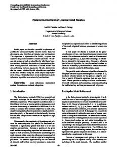
ideas are all heuristic. In the end, we can oer no formal justi cation for the algorithm other than it apparently works quite well, and that it is consistent with the re nement paradigm presented in Section 2. We expect that with more study and experimentation, these heuristics will be improved or better ones developed to replace them. We now give a short numerical illustration of the use of Algorithm Coarsen. We take to be a region in the shape of Lake Superior. The region has a fairly irregular outer boundary and six islands. The initial triangulation used 5927 vertices and is shown in Figure 7. We applied Algorithm Coarsen to this initial mesh, with a target coarse grid containing 300 vertices. Algorithm Coarsen was able to achieve this target value with two restarts, the rst when the mesh had 1412 vertices, and the second when it had 398 vertices. All these meshes are shown in Figure 7. Note that the intermediate meshes with 1412 and 398 vertices do not correspond directly to the triangulations Tk of Section 2, but are simply the mesh as it existed prior to the restart, with many quadrilateral elements to be triangulated. Indeed, this calculation resulted in eight hierarchical levels. Also note that as the coarsening proceeds, the boundary @ is also approximated. The vertex level L(v) for vertices in the (original) ne mesh cannot be determined until Algorithm Coarsen is completed. Even then, L(v) is not necessarily uniquely de ned for all vertices in the mesh, since the coarsening process only yields a partial ordering of the vertices. Of course, it is known that L(v) = 1 for all vertices in the coarse grid. The levels of the remaining vertices must only satisfy

L(v) > maxfL(w1 ); L(w2 )g; where w1 and w2 are the permanent parents of v. Our algorithm for assigning levels to vertices uses both a lower level L(v) and an upper level L (v). For coarse grid vertices, L(v) = L (v) = L(v) = 1. For other vertices, L(v) = maxfL(w1 ); L(w2 )g + 1; where w1 and w2 are the permanent parents of v. This is consistent with vertex levels

assigned by Algorithm Re ne, and can be easily computed by processing vertices in the reverse order in which they were eliminated. Let Lmax = maxv L(v), and let S (v) denote the set of vertices which have v as one of their parents. Then if S (v) = ; L (v) = Lmax ; otherwise, L (v) = min L (v) ? 1; w2S (v)

which is easily computed by processing vertices in the same order in which they were eliminated. For some vertices (at least one at every level) L(v) = L (v)  L(v), while for many others, L(v) < L (v), giving some exibility in level assignment. The assignment of levels has some practical implications, in that the nodal stiness matrix (and implicitly, the hierarchical stiness matrix) are blocked according to the partitioning of vertices into levels. Since the diagonal blocks of the stiness matrix represented in terms of the hierarchical basis are actually computed as part of the preprocessing stages for hierarchical basis iterations, the block structure has some in uence on the work and storage estimates. We have made some experiments using L(v)  L(v) and L(v)  L (v). Choosing L(v)  L (v) results in the diagonal blocks having minimal order at every step, which should result in less work and storage. On typical problems, our empirically observed savings is about 5 ? 10% compared to 12

Fig. 7. The initial triangulation with 5927 vertices, and intermediate grids with 1412, 398, and 300 vertices generated by Algorithm Coarsen.

choosing L(v)  L(v). Since the work and storage requirements are both linear in the number of vertices, this represents a modest, but still signi cant, reduction. We note that this choice need not be optimal in terms of work and storage, although at present, we do not see a way to improve upon it without investing signi cant additional computation. So far, we have noted little dierence in observed rates of convergence for the two choices we have tried, and suspect all assignments consistent with the partial ordering will behave similarly. In Table 1 we record the distribution of vertices among the eight levels for our numerical example of Lake Superior, using both the functions L (v) and L(v) to compute the levels. Here we notice a substantial dierence between the two algorithms. However, this dierence has a negligible impact on the observed rate of convergence. We also note that in our example, the total number of nonzeroes in the upper triangular parts of all the matrices needed for the hierarchical basis multigrid method (see Section 6) is 33198 using levels determined by L (v) and 34971 using L(v). A problem with approximately 6000 vertices created using nested re nement would have 13

level vertices computed vertices computed using L (v) using L(v) 8 3732 21 7 1017 151 6 508 537 5 244 1140 4 89 1860 3 28 1118 2 9 500 1 300 300 Table 1

The distribution of vertices among the eight levels, computed using L (v) and L(v).

a total of approximately 30000 nonzeroes in the corresponding set of matrices. We attribute the increase in our example partly to the suboptimal choices of levels, and partly to edge swapping, which has the eect of increasing the density of nonzeroes in the hierarchical basis stiness matrices. 4. Interpolation Operators for Nonnested Spaces. In this section, we de ne and analyze the interpolation operators used in constructing a hierarchical basis for a sequence of nonnested meshes. We will assume the notation developed in Section 2, and that the sequence of meshes fTk gJk=1 has been generated by Algorithm Re ne. One messy detail of our analysis concerns the approximation of the boundary; all of the triangulations Tk are supposed to approximate the same underlying region , but are able to do so only with dierent degrees of success. We denote by k the region corresponding to the triangulation Tk , and without loss of generality, we assume that

J  . For the remaining regions, we assume that all vertices which lie on @ k also lie on @ . We de ne the bilinear form a(u; w)D , u; w 2 H1 (D), by

a(u; w)D = and the usual L2 inner product by

Z

D

(u; w)D =

ru
rw dx

Z

D

uw dx

for u; w 2 L2 (D). For convenience we set a(u; w) = a(u; w) and (u; w) = (u; w) . We de ne the (level dependent) energy seminorm by jjjujjj2D = a(u; u)D , jjjujjj = jjjujjj , and L2 norm by k u k2D = (u; u)D , k u k=k u k . While it is convenient in this section to work with spaces without boundary conditions, we are careful to insure that the results also apply to the case where the spaces all satisfy homogeneous Dirichlet boundary conditions. Associated with each triangulation Tk , there is a space Mk  H1 ( k ) of continuous piecewise linear polynomials. We let Nk denote the dimension of Mk . Since the triangulations Tk are not nested, the spaces Mk are not nested. However, by construction the vertex sets Xk are nested (Xk  Xi for i > k). We shall assume that all the elements in all the triangulations Tk are shape regular. In particular, we assume that there exists a positive constant , such that G(t)   for 14

all t 2 Tk , 1  k  J , where the quality function G(t) is de ned in (4). We also need a measure of the relative sizes of elements in the various triangulations. Given an element t of size ht , suppose that t~ is the set of elements arising from the application of k steps of Algorithm Re ne to t, with the additional assumption that at least one edge is re ned at each step. Let hmin be the size of the smallest element in the patch t~. Then there exists a constant  = (; ; ),  < 1, such that hmin =ht  k . We next de ne several primitive interpolation operators which play an important k : C ([j j ) 7! Mk denote the role in our hierarchical basis algorithms. First, let I1 usual nodal value interpolant. The interpolation operator Ikk+1 : Mk 7! Mk+1 is a local interpolation operator based on the details of the re nement. Let u 2 Mk ; then we can characterize Ikk+1 u 2 Mk+1 in terms of its values at the set of vertices Xk+1 . First we set Ikk+1 u(v) = u(v) for all v 2 Xk  Xk+1 . For the remaining vertices, we refer to the notation of equation (1). We suppose vr 2 Xk , v` 2 Xk , and v 2 Xk+1 nXk . Then (8) Ikk+1 u(v) = u(vr ) + (1 ? )u(v` ): Notice that Ikk+1 is not pointwise interpolation except for the special case  = 0, that is, when all the meshes are physically as well as logically nested. In this case, Ikk+1 is just the restriction of I1k+1 to Mk . On the other hand, we note from (8) that the value of Ikk+1 u at a vertex v 2 Xk+1 nXk is just a simple linear combination of the values of the function evaluated at v's vertex parents. This keeps the interpolation scheme very local, and extremely simple to implement. Finally, we note that (8) interpolates zero boundary conditions correctly. We next de ne the composite interpolant Ik` : Mk 7! M` for ` > k by Ik` = I``?1 I``??21


Ikk+1 (9) with Ikk = I , and the composite interpolant I~k` : M` 7! M` by

(10) I~k` = Ik` I1k for k < `, with I~`` = I . We now describe the hierarchical basis decomposition for MJ . First note that by construction, each vertex v 2 XJ has a unique level 1  L(v)  J . Using the notation of Algorithm Re ne, and the identi cation X~1  X1 , we have the direct sum decomposition (11) Xk = X~1  X~2 


 X~k for 1  k  J . For convenience, we will order the vertices of the mesh by level; vi for Nk?1 + 1  i  Nk will denote the set of vertices in X~k . For each space Mk , let ki , 1  i  Nk , denote the usual nodal basis functions satisfying ki (vj ) = ij for 1  j  Nk . The hierarchical basis for Mk is de ned inductively in the usual way. First, the hierarchical basis for M1 is just the nodal basis for M1 . For k > 1, we construct a hierarchical basis by interpolating the hierarchical basis for Mk?1 onto Mk using the operator Ikk?1 , and taking the union of the resulting set of functions with the nodal basis functions for the level k nodes (ki , Nk?1 + 1  i  Nk ). We let ik denote the hierarchical basis functions for Mk , ordered using the same scheme as the nodal basis functions. Then we have k k k k Li (12) i = ILi i = I~Li i 15

where we have used the notation Li = L(vi ) to denote the level of vertex vi . We next consider a direct sum decomposition of the space Mk . First, we de ne ~ ki = Iik Mi for 1  i  k. Clearly by (9) these spaces are nested the spaces M k k ~ ~ Mi  Mj  M~ kk  Mk , for i  j  k. By (10), we have M~ ki = I~ik Mk , for 1  i  k. Let Vik = (I~ik ? I~ik?1 )Mk for 1  i  k, with the convention I~0k = 0. Then we have the direct sum decomposition (13) M~ ki = V1k  V2k 


 Vik for 1  i  k. We are especially interested in (13) for the special case i = k = J , MJ  M~ JJ = V1J  V2J 


 VJJ ; since it is the hierarchical decomposition of the space MJ which is of interest to us. Lemma 4.1. Let t 2 Tk be a triangle of size ht , and let t~ be the union of the triangles in T` , ` > k, which arise from the re nement of t as in Algorithm Re ne. Let u 2 Mk , and u~ be the linear polynomial determined by the values of u at the vertices of t, and extended to t~. Then (14) (1 ? c)jjju~jjjt~  jjjIk` ujjjt~  (1 + c)jjju~jjjt~ where c = c(; ; ). Proof. We note that (14) is a local result and does not require quasiuniformity of the mesh; however, this result does depend on the shape regularity of t and each triangle in t~. First, let us consider the linear function u~, which we write as

@u x + @u y + u = ru
v~ + u u~ = @x 0 0 @y

where v~ = (x; y)t , and u0 is constant. Since the gradient of the constant function is zero, and Ik` is exact for constants, without loss of generality, we can assume u0 = 0. Since Ik` is a linear operator, and ru is constant, we have Ik` u = ru
Ik` v~: Let us now examine Ik` v~ using the decomposition (9). We consider rst the simple case Ikk+1 v, where v is a level k +1 vertex with vertex parents vr and v` , in the notation of (1). By (8), we have Ikk+1 v = vr + (1 ? )v` = v ? w so at vertex v the interpolated function value of u is ru
(v ? w). Note that the vector ?w can be interpreted as moving v from its actual location in the nonnested mesh to the location p it would have been had the re nement been nested ( = 0). We also note that wt w  cht . It is simple to see by induction that if v is a vertex of level j in t~

Ik` u = ru
(v ? e)

where ?e is a vector which moves v to its corresponding location in the case of nested re nement ( = 0) of t, and

pt

e e  cht f1 +  + 2 +


+ j?k?1 g  cht (1 ? )?1 : 16

Now let t^ 2 t~ be a triangle in the level ` mesh with vertices vi , nodal basis functions i , and interpolated function values ru
(vi ? ei ), 1  i  3. Then on t^

rIk` u = ru ?

3 X

i=1

ru
ei ri

= ru ? ru
f(e2 ? e1 )r2 + (e3 ? e1 )r3 g: Now we make a critical observation, that the vectors e2 ? e1 and e3 ? e1 denote the change in shape in element t^ relative to the case  = 0, as opposed to a change in location; in eect, we have subtracted the translation common to all three vertices. Since t^ and the corresponding triangle in the case of nested re nement are both shape regular, we must have for i = 2; 3, p

(ei ? e1)t (ei ? e1 )  cht^

Since jri j  cht?^ 1 , we have immediately

(1 ? c)jjju~jjjt^  jjjIk` ujjjt^  (1 + c)jjju~jjjt^: The result now follows by summing over t^ 2 t~. Since Lemma 4.1 is a critical result in our analysis, we pause here to give a numerical illustration. We consider a single element t, and re ne 9 levels as in Figure 1 E, with  =  = 0:5, and  =  = 0:1,  =  = 0:05, and  =  = 0:01. In Figure 8, we show the original element t and the regions t~ for k + 1  `  k + 5 and  = :1. (the more re ned regions have too many elements to be resolved in a small picture). In Figure 9, we show the corresponding contour maps for the function u = ki (one of the nodal basis functions for t) and the corresponding functions Ik` u. Finally, in Table 2, we show the function jjjIk` ujjjt~=jjju~jjjt~ ? 1 for k  `  k + 9, where one can see clearly the predicted behavior c.

`

k k+1 k+2 k+3 k+4 k+5 k+6 k+7 k+8 k+9

triangles vertices  = :1  = :05  = :01 1 3 0.0 0.0 0.0 4 6 -2.77(-2) -1.41(-2) -2.87(-3) 16 15 -2.00(-2) -1.21(-2) -2.79(-3) 64 45 -1.54(-2) -1.10(-2) -2.75(-3) 256 153 -0.96(-2) -9.64(-3) -2.69(-3) 1024 561 -0.37(-2) -8.26(-3) -2.63(-3) 4096 2145 0.25(-2) -6.89(-3) -2.59(-3) 16384 8385 0.89(-2) -5.52(-3) -2.53(-3) 65536 33153 1.59(-2) -4.01(-3) -2.48(-3) 262144 131841 2.23(-2) -2.71(-3) -2.32(-3) Table 2

The function jjjIk` ujjjt~=jjju~jjjt~ ? 1 for k  `  k + 9 and  = :1; :05; :01.

Lemma 4.2. Let t 2 Tk be a triangle of size ht , and let t~ be the union of the triangles in T` , ` > k, which arise from the re nement of t as in Algorithm Re ne. k u, and let w~ be the linear polynomial determined by the Let u 2 M` and w = I1

values of w at the vertices of t, and extended to t~. Then

(15)

p jjjw~jjjt~  C ` ? kjjjujjjt~ 17

Fig. 8. The element t and t~ for ` = k + 1; k + 2;


; k + 5, and  = :1

Fig. 9. Contour maps for the function u and

Ik` u for ` = k + 1; k + 2;


; k + 5, and  = :1

18

for C = C (; ; ). Proof. Since w 2 Mk , w is just a linear polynomial on t. As in the proof of Lemma 4.1, let vi , 1  i  3, denote the vertices of t. Then, noting w(vi ) = u(vi ), we have,

jjjw~jjjt~  C max jw(vi )j = C max ju(vi )j  C k u k1;t~ : i i Let hmin denote the size of the smallest triangle in t~. Then 



k u k21;t~ C log hht jjjujjj2t~  C log k?` jjjujjj2t~  C (` ? k)jjjujjj2t~: min ?




This completes the proof. Theorem 4.3. Let u 2 M` and let ` > k. Then p jjjI~k` ujjj `  C ` ? kjjjujjj ` (16)

for C = C (; ; ). Proof. Let t 2 Tk , and let t~ be the union of triangles in T` which arise from k u and let w~ be the linear the re nement of t as in Algorithm Re ne. Let w = I1 polynomial determined by the values of w at the vertices of t and extended to t~. Then by Lemmas 4.1 and 4.2, jjjI~k` ujjjt~ = jjjIk` wjjjt~  (1 + c)jjjp w~jjjt~  C (1 + c) ` ? kjjjujjjt~:

The result (16) follows by summing over t 2 Tk . The next lemma shows that a bound on the interpolant as in (16) in essentially equivalent to a strengthened Cauchy inequality [3] [12]. Lemma 4.4. Suppose M = V  W , and let I denote the interpolation operator de ned as follows: if u = v + w 2 M, v 2 V , and w 2 W , then I (u) = v. Then (17)

jjjI (u)jjjD  C jjjujjjD

if and only if

ja(v; w)D j  jjjvjjjD jjjwjjjD for < 1 and for all v 2 V and w 2 W . (18)

Proof. First, we assume (18) in order to prove (17). Let u = v + w, v 2 V , w 2 W . Then

jjjujjj2D = a(v + w; v + w)D = jjjvjjj2D + jjjwjjj2D + 2a(v; w)D  jjjvjjj2D + jjjwjjj2D ? 2 jjjvjjjD jjjwjjjD  (1 ? 2 )jjjvjjj2D : Therefore

jjjI (u)jjjD  p 1 2 jjjujjjD : 1? 19

Now we assume (17) to show (18). It suces to take jjjvjjjD = jjjwjjjD = 1. Then, from (17) jjjv ? wjjj  1 jjjvjjj = 1 : D

Thus,

D

C

C

a(v; w)D = 21 jjjvjjj2D + 21 jjjwjjj2D ? 12 jjjv ? wjjj2D  1 ? 2C1 2 : Theorem 4.5. Let u = v + w 2 Mk , with v 2 V1k  V2k 


 Vik

and

w 2 Vik+1  Vik+2 


 Vkk for 1  i < k. Then

(19)





ja(v; w) j  1 ? k C? i jjjvjjj jjjwjjj : k

k

k

Proof. Apply Lemma 4.4 and Theorem 4.3. We next prove another strengthened Cauchy inequality. Theorem 4.6. Let u 2 Vi` and w 2 Vk` . Then there exists a constant C =  C (; ; ), such that, for  suciently small,

(20)





ja(u; w) j  C ji?kj=2 +  jjjujjj jjjwjjj : `

`

`

Proof. Our proof follows closely the proof of Lemma 4.1. For convenience, suppose

i < k, and let t 2 Ti and t~ denote the set of elements in T` resulting from the re nement of t. Let u~ be the linear polynomial characterized by the values of u at the vertices of t, and set u = ru~
(v ? e) = u~ + z , as in the proof of Lemma 4.1. As in the proof of Lemma 4.1, we may set the constant u~0 = 0. We rst consider the term a(~u; w)t and note Z @ u~ w dx a(~u; w)t~ = @n @ t~ where n is the unit normal. Note that w  0 on edges of @ t~ which are level k ? 1 or less, and w = 0 at all vertices in t~ of level k ? 1 or less. Thus w  0 on any element in t~ not containing at least one vertex of level k or larger, and where w 6= 0, it must be oscillatory. Let hi denote the size of t~, and hk denote size of elements of level k which came from the re nement of t. Then hk =hi  C k?i , and 20

!1=2 Z

1=2 @ u~ 2 dx 2 dx ja(~u; w)t~j  w @ t~ @n @ t~  pch jjju~jjjt~ phhk jjjwjjjt~ i i j i ? k j = 2  c  jjjujjjt~ jjjwjjjt~: Here we have estimated jjju~jjjt~ using Lemma 4.1 assuming that 1 ? c > 0 in (14), and used standard trace and inverse estimates for the terms involving w. Using the 

Z





arguments of Lemma 4.1 once more, we have ja(z; w)t~j  C jjjujjjt~ jjjwjjjt~: Combining these two estimates, and summing over t 2 Ti (in eect, summing over the re ned patches t~ ) leads to the estimate (20). Our nal theorem is P Theorem 4.7. Let u 2 Vk` , u = i Ui i` , where the i` are the hierarchical basis functions described above, and k > 1. Then there exist constants Ci = Ci (; ; ), 1  i  2, such that (21)

C1 jjjujjj2 ` 

X

i

Ui2 jjj i` jjj2 `  C2 jjjujjj2 ` :

Proof. The left inequality in (21) is a simple exercise using the triangle inequality, and the fact the support of i` can intersect the support of only a xed number of hierarchical basis functions of the same level, and is true even in the case k = 1. The right inequality is more dicult, and will be proved elementwise for t 2 Tk . Since Tk came from the re nement of Tk?1 , all of the elements must be of the patterns shown in Figure 1. As usual, we will let t~ denote the patch of elements in T` which arise from the subsequent re nement of t. In Figure 1 A, no edges were re ned and the single element has all vertices with level less than k; thus u  0 on t~, and there is nothing to prove. In Figure 1 B, there is one level k vertex, and hence one nonzero basis function, say i`1 . If t~ corresponds to one of the two elements t 2 Tk arising from such a re nement then jjjujjj2t~ = Ui21 jjj i`1 jjj2t~, and again the proof is trivial. In Figure 1 C, one of the three elements has only one nonzero basis function, and is similar to the case of Figure 1 B. The remaining elements have two nonzero basis functions, say i`1 and i`2 . To obtain a local bound, we are led to study the 2  2 eigenvalue problem    0 jjj i`1 jjj2t~ a( i`1 ; i`2 )t~   Ui1  =   jjj i`1 jjj2t~ Ui1 Ui2 a( i`1 ; i`2 )t~ jjj i`2 jjj2t~ 0 jjj i`2 jjj2t~: Ui2 The eigenvalues are  = 1  , where ja( ` ; ` ) j  = ` i1 i2` t~ :

jjj i1 jjjt~jjj i2 jjjt~

We will show  < 1, depending only on ,  and . Following the pattern of Lemma 4.1, we let i`1 = ~i`1 + zi1 , where ~i`1 is the linear polynomial based on the 21

values at the vertices of t (in this case, ~i`1 = 0 at two nodes and ~i`1 = 1 at the third). We make an analogous decomposition for i`2 . Note that ~i`2 = 1 at one of the two vertices where ~i`1 = 0. Now let t^ 2 T` be one of the triangles in the set of elements making up t~. Then r i`1 and r i`2 are constant on t^ and essentially small perturbations of r ~i`1 and r ~i`2 , respectively. By shape regularity combined with their de nitions we must have the strengthened Cauchy inequality

jr

q

` ` i1
r i2 j  t^

r

` ` i1
r i1

q

r

` ` i2
r i2

leading directly to the estimate

ja( i`1 ; i`2 )t^j  t^jjj i`1 jjjt^jjj i`2 jjjt^: Taking  = maxt^ t^ and summing over t^ complete the estimate in this case. For re nement as in Figure 1 D, all four elements have two nonzero basis functions and are covered by the preceding argument. For re nement as in Figure 1 E, three of the four elements in Tk have two nonzero basis functions, while the middle element has three nonzero basis functions. The argument above will fail for such elements, as the analogous 3  3 eigenvalue problem will have one zero eigenvalue and two positive eigenvalues. On the other hand, such elements only occur in the situation shown in Figure 1 E, where they are surrounded by three elements, each having only two nonzero basis functions. Let t0 denote the center element with three nonzero basis functions, and let t1 , t2 and t3 denote the other three triangles, each with two nonzero basis functions. Let i`1 , i`2 , and i`3 denote the three basis functions. Suppose i`1 has support in t2 and t3 as well as t0 . Then using arguments similar to those in Lemma 4.1, it is straightforward to show

c1 jjj i`1 jjj2t~0  jjj i`1 jjj2t~2 + jjj i`1 jjj2t~3  c2 jjj i`1 jjj2t~0 so that we can control the behavior of the center element though the surrounding elements which have only two nonzero basis functions. Similar estimates apply to the other two basis functions. These can be combined to show

Ui21 jjj i`1 jjj2t~0 + Ui22 jjj i`2 jjj2t~0 + Ui23 jjj i`3 jjj2t~0  C jjjujjj2t~0 [t~1 [t~2 [t~3 : Now, by combining all cases, and summing over t 2 Tk , we obtain the right hand

inequality in (21). We close this section with a few remarks. The rst concerns the issue of dynamic edge swapping. We note that under appropriate assumptions, one can show jjjS ujjjD  jjjujjjD where S is an \edge swapping" operator. For example, if we were to allow dynamic edge swapping once, say only on the nest triangulation TJ , we would have growth like C (1 + c), C > 1 in Lemma 4.1. This could be generalized to any xed number p of levels on which edge swapping is allowed with growth like C p (1 + c)p . However, if we allowed dynamic edge swapping on all levels (p = J ), clearly the growth would not be acceptable. We emphasize that we do not believe that dynamic edge swapping is harmful to the coarsening (or re nement) process; indeed, it is a critical part of the restart step of Algorithm Coarsen, and from our practical experience in this context, has little if any observed eect on the convergence of iterations using hierarchical basis preconditioners. It just seems that the theory developed in this section is not yet mature enough to adequately explain this observed behavior. 22

Our second remark concerns the eect of a variable coecient in the enery inner product. Suppose that

a~(u; w)D =

Z

D

aru
rw dx

where a = a(x; y) is a piecewise smooth, positive, bounded function on D. Let t 2 T1 and t~ be the set of elements in TJ resulting from the re nement of t. Let 0 < at~  a(x; y)  at~ on t~ and set  = maxt~ at~=at~. Then most constants in our analysis would depend on  as well as ,  and . We note that  is a locally de ned quantity, and depends only on the variation of a(x; y) on ne grid patches of elements corresponding to coarse grid triangles. For example, if a is a piecewise constant, it will have no eect on our estimates as long as the interfaces where a has jumps are modeled in the coarse triangulation. This is independent of the sizes of the jumps, and is of course exactly similar to the behavior of hierarchical basis decompositions on sequences of nested meshes. However, it is interesting to note that we do not have to approximate these interfaces exactly on the coarse grids, just as we do not have to approximate the boundary @ exactly on the coarse grids. Indeed the same basic re nement rule applies to both interfaces and boundaries: when an interface (boundary) edge is re ned, the new vertex should be placed on the interface (boundary). Neither the original interface (boundary) edge or its two children edges are required to coincide exactly with the interface (boundary). This explains our motivation for giving boundary and interface vertices similar special treatment in assigning tentative vertex parents in Algorithm Coarsen. 5. Some Hierarchical Basis Preconditioners. In this section, we will analyze block Jacobi and block symmetric Gauss-Seidel iterations using the hierarchical decomposition

MJ = V1J  V2J 


 VJJ de ned in Section 4. However, for convenience in this section, we assume that the space MJ  H01 ( ). Satisfying the Dirichlet boundary conditions amounts to excluding basis functions associated with boundary vertices from the subspace. In order to avoid the notational explosion involved with this change, we adopt the same notation as in Section 4, and simply remark that many symbols have slightly altered meanings to accommodate the boundary conditions. One important change is that jjj
jjj becomes a strong norm instead of a seminorm. As before, we let f ik gNi=kNk?1 +1 denote the hierarchical basis functions for the level-k vertices in TJ . Then the stiness matrix A, represented in the hierarchical basis, is expressed as the symmetric, positive de nite block J  J matrix 2

(22)

6

A11 A12


A1J A21 A22 A2J

A = 664 .. . . . .. . . AJ 1 AJ 2


AJJ

3 7 7 7 5

where Akk is the (Nk ? Nk?1 )  (Nk ? Nk?1 ) matrix of energy inner products involving just the level-k basis functions. We set (23)

A = L + D + Lt 23

where

2 6

A11

D = 664 and

2

3

A22

...

AJJ

0

3

0

3

7 7 7 5

7 6 A21 0 7 L = 664 .. . . . 75 : . AJ 1 AJ 2


0 The block diagonal matrix D is further decomposed as D = d + ` + `t , where 3 2 A11 7 6 d22 7 d = 664 7 ... 5 dJJ dii = DiagAii , and 2 6

` = 664

`22

...

`JJ

7 7 7 5

is lower triangular. We rst analyze the block Jacobi preconditioner d. This is similar to the hierarchical basis method of Yserentant [29]. Theorem 5.1. Let A = L + D + Lt and D = ` + d + `t as de ned above. Then there exist positive constants Ci = Ci (; ; ), i = 1; 2, such that (24)

t dU C1 (1 + J )?1  UUt AU  C2 J 2

for U 6= 0. Proof. The upper bound in (24) is similar to the hierarchical basis preconditioner for the case of nested meshes. The lower bound in the nested case does not have the term (1 + J )?1 . However, for typical choices of  and J , this term is eectively bounded by a constant, so as a practical matter, the bound (22) does not dier signi cantly from the nested mesh case. We begin our proof by writing the Rayleigh quotient in (24) as

U tdU = U t DU U t dU U t AU U t AU U t DU and will estimate each of the terms separately. Let u 2 MJ correspond to U in (24). Then the Rayleigh quotient U t DU=U tAU can be written as P U t DU = Jk=1 jjjzk jjj2 U t AU jjjujjj2 24

where zk = (I~kJ ? I~kJ?1 )u. Applying Theorem 4.3 for the upper bound, and Theorem 4.6 for the lower bound, we have t 2 c1 (1 + J )?1  UU tDU AU  c2 J :

For the Rayleigh quotient U t dU=U t DU , we can apply Theorem 4.7 to see t dU c1  UUt DU  c2 :

Combining these estimates proves (24). We next consider the symmetric block Gauss-Seidel preconditioner using symmetric Gauss-Seidel \inner iterations", an algorithm similar to the Hierarchical Basis Multigrid Method [4] [1]. We begin with a few preliminary lemmas. Lemma 5.2. Let A = L + D + Lt and let B~ = (D + Lt )D?1 (D + L) = A + Lt D?1 L. Then there exists a positive constant C = C (; ; ), such that t~ 2 1  UU tBU (25) AU  1 + 0  CJ for U 6= 0, and

W t DW : 0 = max U 6=0 U t AU DW = LU:

Proof. The preconditioner B~ is essentially that for block symmetric Gauss-Seidel, assuming that all linear systems involving the diagonal blocks Aii are solved exactly. The lower bound and upper bound 1 + 0 follow immediately from the de nition of B~ and the fact that LtD?1 L is positive semide nite. To estimate 0 , let u 2 MJ correspond to U in (25). Then, in nite element notation, PJ

2 k=2 jjjwk jjj 0 = max u6=0 jjjujjj2

where

a(wk ; ) = a(I~kJ?1 u; )

for all  2 VkJ . Taking  = wk in this relation and applying Theorem 4.3 leads to p jjjwk jjj  jjjI~kJ?1 ujjj  C J ? k + 1jjjujjj

which immediately implies 0  CJ 2 . Lemma 5.3. Let D = ` + d + `t and let D~ = (d + `t )d?1 (d + `) = D + `t d?1 `. Then there exists a positive constant C = C (; ; ), such that t DU ~ (26)  1 + 1  C 1  UU t DU 25

for U 6= 0, and

W t dW 1 = max U 6=0 U t DU dW = `U: Proof. The preconditioner D~ summarizes the symmetric Gauss-Seidel inner iterations. The proof follows the pattern of that for Lemma 5.2, using Theorem 4.7 in place of Theorem 4.3. The preconditioner for the Hierarchical Basis Multigrid Method using symmetric Gauss-Seidel inner iterations is given by B = (D~ + L)t (2D~ ? D)?1 (D~ + L) (27) = A + (D ? D~ + L)t (2D~ ? D)?1 (D ? D~ + L) = A + (L ? Z )t (D + 2Z )?1 (L ? Z )

where Z = `t d?1 ` [4] [1]. Theorem 5.4. Let A = L + D + Lt and let B be given by (27). Then there exists a positive constant C = C (; ; ), such that (28)

t

2 1  UU tBU AU  CJ

for U 6= 0. Proof. We begin by noting that the matrix (L ? Z )t (D + 2Z )?1(L ? Z ) is symmetric, positive semide nite. This gives a lower bound of of 1  U t BU=U tAU and an upper bound of the form U t BU=U t AU  1 + , where

U t (L ? Z )t (D + 2Z )?1(L ? Z )U  = max U 6=0 U t AU = k (D + 2Z )?1=2 (L ? Z )A?1=2 k2`2   k (D + 2Z )?1=2 D1=2 k`2 k D?1=2 LA?1=2 k`2

2

+ k (D + 2Z )?1=2 ZD?1=2 k`2 k D1=2 A?1=2 k`2 : Now k (D +2Z )?1=2D1=2 k`2 = 1, since Z = `td?1 ` is symmetric, positive semidefinite, while k D?1=2 LA?1=2 k`2 = 0  CJ 2 and k D1=2 A?1=2 k`2  CJ 2 using Lemma 5.2 and Theorem 5.1, respectively. Finally, from Lemma 5.3, k (D + 2Z )?1=2 ZD?1=2 k`2  p1 k D?1=2 ZD?1=2 k`2 = p1  C: 2 2 Combining these estimates, we see that   CJ 2 , just as in the basic block symmetric Gauss-Seidel iteration. We next formally de ne algorithms similar to BPX [10] and regular multigrid algorithms based on our decomposition. We will use the ideas of Griebel [15] [14], who characterizes these methods as particular iterations applied to an enlarged, semidefinite system. For each vertex vi 2 XJ , let L(vi )  Li denote the vertex level of vi 26

and E (vi )  Ei denote the maximum edge level of any edge in EJ having vi as an endpoint. Clearly 1  Li  Ei  J . With each vertex vi 2 XJ , we associate a set of one or more basis functions given by ik = I~kJ i

for Li  k  Ei . Here i  Ji (= iEi ) are just the nodal basis functions for MJ , and iLi  iJ are the usual hierarchical basis functions for MJ . We next de ne the subspaces V~kJ by  V~kJ = span ik : Note that VkJ  V~kJ and

MJ = V~1J + V~2J +


+ V~JJ : We note that this is not a direct sum decomposition as in the case of hierarchical basis methods. We can now form a block J  J , symmetric, positive semide nite stiness matrix A given by 2

(29)

6

A11 A12


A1J A21 A22 A2J

A = 664 .. . . . .. . . AJ 1 AJ 2


AJJ

3 7 7 7 5

where Akk involves energy inner products of the ik . If the enlarged nite element system is AU = B, then Griebel shows that any solution U of the singular system corresponds to the unique nite element solution u 2 MJ . Within this framework, the BPX method is just a block Jacobi preconditioner analogous to the Hierarchical Basis preconditioner analyzed in Theorem 5.1, but applied to the matrix A. Similarly, the block symmetric Gauss Seidel Preconditioner, using symmetric Gauss Seidel as an inner iteration as in Theorem 5.4, is just a particular multigrid V -cycle using symmetric Gauss-Seidel as smoother when applied to the matrix A. In the case of nested meshes, both BPX and regular multigrid V -cycle have been shown to have condition numbers which are bounded independent of the number of levels J [23] [24] [28] [30] [8]. Furthermore, those bounds apply in three as well as two space dimensions. Our analysis of these methods, based on the results of Section 4, is essentially the same as Theorems 5.1 and 5.4, and has neither of these properties. On the one hand, one should expect these BPX and multigrid like preconditioners to outperform hierarchical basis and hierarchical basis multigrid preconditioners, respectively, since unknowns associated with certain grid points are processed on several levels, rather than only one. On the other hand, our subspace decomposition is based on the approximate pointwise interpolation operators I~kJ rather than L2 projections, so it is problematic that these preconditioners could be shown to achieve the same sorts of condition numbers as their counterparts based on nested re nement. 27

6. Implementation Issues. In this section we discuss several important aspects of the practical implementation of the hierarchical basis multigrid and other hierarchical basis preconditioners. The most dicult issue is that, in typical applications, the stiness matrix is assembled using the nodal basis functions rather than the hierarchical basis. The reason is that the nodal basis functions have small supports, only three such functions are nonzero in any given element of the ne mesh, and therefore the stiness matrix represented in the nodal basis is both easy to assemble and very sparse. In contrast, since hierarchical basis functions have supports of varying sizes, depending on the level, the stiness matrix represented in the hierarchical basis is more complicated to assemble and much less sparse the that of the nodal basis (although better conditioned). To give a theoretical analysis of the method as in Sections 4 and 5, it is sucient to assume the linear system is assembled in the hierarchical basis. However, to eciently implement the method, one must assemble the stiness matrix with respect to the nodal basis, and then implement the hierarchical basis iteration in an implicit fashion. It is through this aspect of their implementation that the connection between hierarchical basis methods and multigrid methods becomes clear. We will give a simple illustration of how this is done, by considering in detail the case of two levels. We write the linear system A^U^ = F^ , constructed with respect to the standard nodal basis, in block form as  ^11 A^12   U^1   F^1  A (30) A^21 A^22 U^2 = F^2 : Here we have assumed a partitioning corresponding to the two level hierarchical decomposition. The system (30) is related to the hierarchical basis system (31)



A11 A12 A21 A22







U1 = F1 F2 U2



via a nonsingular matrix S which transforms the representation of a nite element function with respect to the hierarchical basis into its representation with respect to a nodal basis. S has the block structure   I 0 S= (32) :

R I

The o-diagonal entries of S are zero except for at most two nonzeroes in each row of R. Let vi have Li = 2, and let v` and vr be the vertex parents of vi . Then the two nonzero coecients in R for row i are Sir =  and Si` = 1 ? , where  is the interpolation coecient de ned in (4) and (1). Using (32) we relate the matrices A and A^ , the right hand sides F and F^ , and solutions U and U^ by ^ A = S t AS F = S t F^ U^ = SU: Blockwise this gives

A11 = A^11 + Rt A^21 + A^12 R + Rt A^22 R A12 = A^12 + Rt A^22 28

= A^21 + A^22 R = A^22 = F^1 + Rt F^2 = F^2 = U1 = RU1 + U2 : A single iteration cycle of the hierarchical basis multigrid method, expressed in the current notation, is given below. First, we approximately solve (33) A22 W2 = F2 using a symmetric Gauss-Seidel inner iteration. To avoid introducing more notation, we denote the approximate solution by W2 . We then form the level-1 hierarchical basis residual G1 = F1 ? A12 W2 as (34) G1 = (F^1 ? A^12 W2 ) + Rt (F^2 ? A^22 W2 ): Next, we solve (35) A11 W1 = G1 by a direct method, and set W^ 1 = W1 . Next, form the level-2 hierarchical basis residual G2 = F2 ? A21 W1 ? A22 W2 as (36) G2 = F^2 ? A^21 W^ 1 ? A^22 (RW1 + W2 ) Next, we approximately solve (37) A22 Z2 = G2 using a symmetric Gauss-Seidel inner iteration, denote the approximate solution by Z2 , and set (38) W^ 2 = RW1 + W2 + Z2 : Careful inspection of (33)-(38) shows the hierarchical basis method to be closely related to a standard multigrid V-cycle. Equations (33) and (37) correspond to multigrid smoothing steps, except that only the level-2 unknowns (W2 and Z2 ) are smoothed, rather than all unknowns. After the rst (pre) smoothing step in (33), the approximate solution with respect to the nodal basis is     U^1  0 : W2 U^2

A21 A22 F1 F2 U^1 U^2

In (34), forming the residual vector G1 consists of forming the ne grid residuals after smoothing with respect to the nodal basis   F^1 ? A^12 W2 F^2 ? A^22 W2 and making a \ ne-to-coarse" grid transfer (multiply by Rt) to compute the residual with respect to the hierarchical basis for the level-1 unknowns. Equation (35) is the 29

standard multigrid coarse grid correction, done by direct methods for our case J = 2, but more generally handled by recursion for J > 2. In (36) we update the nodal basis solution as     U^1  W^ 1 RW1 + W2 U^2 using \coarse-to- ne" grid interpolation (multiply by R), and form the ne grid residual G^ 2 . After the second (post) smoothing step (37), the approximate solution with respect to the nodal basis is     U^1  W^ 1 : U^2 W^ 2 To carry out this iteration, we need the matrices A^22 = A22 , A^12 , and A11 , all of which are sparse. The matrices A^12 and A^22 are just blocks of the original stiness matrix computed with respect to the nodal basis. In the case of nested re nement, A11 is just the stiness matrix formed from energy inner products of the coarse grid nodal basis functions. In our case, A11 has a similar sparsity pattern to that of the nested case, but the basis functions involved are the nodal basis functions for the coarse grid interpolated onto the ne grid using (4). However, we never have to explicitly form or compute with these basis functions; rather we compute A^ as in (30), using the usual nodal basis, and form A11 = A^11 + Rt A^21 + A^12 R + Rt A^22 R. The matrix R is also sparse; its sparsity structure is known through the vertex parents for each vertex, and the numerical values for each row ( and 1 ? ) can be conveniently stored in one or two linear arrays of order NJ . For more than two levels, the procedure is implemented recursively, which aects only equation (35). Matrix A11 is recursively decomposed into pieces corresponding to coarser levels, but with the same structure as the basic two level matrices described above. We close this section with a numerical example, using the hierarchical basis multigrid method applied to the Lake Superior example of Section 3. The partial dierential equation we solved was

?
u = 1

in ; on @ :

u = 0

The application of Algorithm Coarsen with a target value of 300 vertices in the coarse grid triangulation resulted in eight hierarchical basis levels, which we de ned using the function L(v)  L (v). The graphs of the resulting stiness matrices (similar to A11 above, but now generated recursively for each of the hierarchical basis levels) are shown in Figures 10 and 11. As is standard in sparse matrices, each edge in the graph corresponds to a nonzero in the upper triangular part of the stiness matrix. Perhaps the most striking feature of these graphs is that, with the exception of case of the original mesh, none of the graphs are triangulations. This is partly due to a suboptimal choice of levels, and partly due to edge swapping. For example, if the mesh with 1412 vertices in Figure 7 was one of the meshes (it is not) then the graph of the mesh would be the graph of the stiness matrix, with the remark that for each quadrilateral element, both diagonal edges must be added. In eect, edge swapping creates nonzeroes in the stiness matrix 30

connecting all four vertices involved in the swap. This eect propagates through subsequent edge swaps, so the matrix graphs become progressively more distant from the underlying triangulations. The extra edges due to swapping also increase slightly the overall work and storage involved in the algorithm, as noted in Section 3.

Fig. 10. Graph of the initial stiness matrix with 5927 vertices, and graphs of the hierarchical basis matrices with 2195, 1178 and 670 vertices.

is

The convergence history is shown on the right in Figure 12. The quantity plotted 

 k r k k k = log k r k ; 0 where rk is the residual at iteration k and k
k is the `2 norm. Standard conjugate

gradient acceleration was used. From the data points, we estimate by least squares that the convergence rate is approximately :37, which is fairly typical of this particular iterative method applied to a similar problem on a sequence of re ned meshes. REFERENCES 31

Fig. 11. Graphs of the hierarchical basis matrices with 426, 337, 309, and 300 vertices.

[1] R. E. Bank, Hierarchical preconditioners for elliptic partial dierential equations, in Large Scale Matrix Problems and the Numerical Solution of Partial Dierential Equations (J. Gilbert and D. Kershaw, eds.), Oxford University Press, 1994, pp. 121{155. , PLTMG: A Software Package for Solving Elliptic Partial Dierential Equations, Users' [2] Guide 7.0, Frontiers in Applied Mathematics, SIAM, Philadelphia, 1994. [3] R. E. Bank and T. F. Dupont, Analysis of a two level scheme for solving nite element equations, Tech. Rep. CNA-159, Center for Numerical Analysis, University of Texas at Austin, 1980. [4] R. E. Bank, T. F. Dupont, and H. Yserentant, The hierarchical basis multigrid method, Numer. Math., 52 (1988), pp. 427{458. [5] R. E. Bank, A. H. Sherman, and A. Weiser, Re nement algorithms and data structures for regular local mesh re nement, in Scienti c Computing (Applications of Mathematics and Computing to the Physical Sciences) (ed. R. S. Stepleman), North Holland, 1983, pp. 3{17. [6] R. E. Bank and J. Xu, The hierarchical basis multigrid method and incomplete LU decomposition, in Proceedings of Seventh International Conference on Domain Decomposition. (ed. D. Keyes and J. Xu), AMS, Providence, Rhode Island, 1994, pp. 163{173. , A hierarchical basis multigrid method for unstructured meshes, in Fast Solvers for Flow [7] Problems. Proceedings of the Tenth GAMM-Seminar Kiel, (Notes on Numerical Mathematics, vol. 49, W. Hackbusch and G. Wittum, eds.), Vieweg-Verlag, Braunschweig, 1995, pp. 1{13. 32

Fig. 12. Convergence history for HBMG with conjugate gradient acceleration.

[8] F. Bornemann and H. Yserentant, A basic norm equivalence for the theory of multigrid methods, Numer. Math., 64 (1993), pp. 455{476. [9] J. Bramble, J. Pasciak, and J. Xu, The analysis of multigrid algorithms with non-imbedded spaces or non-inherited quadratic forms, Math. Comp., 56 (1991), pp. 1{43. [10] J. H. Bramble, J. E. Pasciak, and J. Xu, Parallel multilevel preconditioners, Math. Comp., 55 (1990), pp. 1{22. [11] T. F. Chan and B. F. Smith, Domain decomposition and multigrid algorithms for elliptic problems on unstructured meshes, in Proceedings of Seventh International Conference on Domain Decomposition. (ed. D. Keyes and J. Xu), AMS, Providence, Rhode Island, 1994, pp. 175{189. [12] V. Eijkhout and P. Vassilevski, The role of the strengthened Cauchy-Buniakowskii-Schwarz inequality in multilevel methods, SIAM Review, 33 (1991), pp. 405{419. [13] A. George and J. Liu, Computer Solution of Large Sparse Positive De nite Systems, Prentice Hall, Englewood Clis, NJ, 1981. [14] M. Griebel, Multilevel algorithms considered as iterative methods on semide nite systems, SIAM J. Sci. Comput., 15 (1994), pp. 547{565. , Multilevelmethoden als Interationsverfahren Erzeugendensystemen, B. G. Teubner, [15] Stuttgart, 1994. [16] M. Griebel and P. Oswald, Remarks on the abstract theory of additive and multiplicative Schwarz algorithms, Tech. Rep. TUM-19314, Institut fur Informatik, Technische Universitat Munchen, 1993. [17] W. Hackbusch, Multigrid Methods and Applications, Springer-Verlag, Berlin, 1985. [18] W. Hackbusch and G. Wittum, eds, Incomplete Decompositions - Algorithms, Theory and Applications, Notes on Numerical Fluid mechanics, vol. 41, Vieweg, Braunschweig, 1993. [19] R. H. W. Hoppe and R. Kornhuber, Adaptive multilevel methods for obstacle problems, SIAM J. Numer. Anal., (to appear). [20] R. Kornhuber, Monotone multigrid methods for variational inequalities I, Numer. Math., (to appear). [21] D. J. Mavriplis, Multigrid techniques for unstructured meshes, Tech. Rep. 95-27, Institute for Computer Applications in Science and Engineering, Hampton, Virginia, 1995. [22] W. F. Mitchell, A comparison of adaptive re nement techniques for elliptic problems, ACM Trans. Math. Soft., 15 (1989), pp. 326{347. [23] P. Oswald, On discrete norm estimates related to multigrid preconditioners in the nite element method, in Proceedings of the International Conference on Constructive Theory of Functions, Varna, 1991. 33

[24] [25] [26] [27] [28] [29] [30] [31]

, Multilevel Finite Element Approximation. Theory and Applications, B. G. Teubner, Stuttgart, 1994. M. C. Rivara, Algorithms for re ning triangular grids suitable for adaptive and multigrid techniques, Int. J. Numer. Meth. Eng., 20 (1984), pp. 745{756. D. J. Rose, A graph theoretic study of the numeric solution of sparse positive de nite systems, in Graph Theory and Computing, Academic Press, New York, 1972. J. Xu, Theory of Multilevel Methods, PhD thesis, Cornell University. Report AM-48, Penn State, 1989. , Iterative methods by space decomposition and subspace correction, SIAM Review, 34 (1992), pp. 581{613. H. Yserentant, On the multi-level splitting of nite element spaces, Numer. Math., 49 (1986), pp. 379{412. , Old and new convergence proofs for multigrid methods, in Acta Numerica, Cambridge University Press, 1992. S. Zhang, Multilevel Iterative Techniques, PhD thesis, Pennsylvania State University, Department of Mathematics Report 88020, 1988.

34