IOS Press. An algorithm for correcting mislabeled data. Xinchuan Zeng and Tony R. .... The updating rule modifies the class probability vectors of mislabeled ...
Intelligent Data Analysis 5 (2001) 491–502 IOS Press
491
An algorithm for correcting mislabeled data Xinchuan Zeng and Tony R. Martinez Computer Science Department, Brigham Young University, Provo, UT 84602, USA E-mail: {zengx,martinez}@cs.byu.edu Received 12 June 2001 Revised 22 July 2001 Accepted 25 August 2001 Abstract. Reliable evaluation for the performance of classifiers depends on the quality of the data sets on which they are tested. During the collecting and recording of a data set, however, some noise may be introduced into the data, especially in various real-world environments, which can degrade the quality of the data set. In this paper, we present a novel approach, called ADE (automatic data enhancement), to correct mislabeled data in a data set. In addition to using multi-layer neural networks trained by backpropagation as the basic framework, ADE assigns each training pattern a class probability vector as its class label, in which each component represents the probability of the corresponding class. During training, ADE constantly updates the probability vector based on its difference from the output of the network. With this updating rule, the probability of a mislabeled class gradually becomes smaller while that of the correct class becomes larger, which eventually causes the correction of mislabeled data after a number of training epochs. We have tested ADE on a number of data sets drawn from the UCI data repository for nearest neighbor classifiers. The results show that for most data sets, when there exists mislabeled data, a classifier constructed using a training set corrected by ADE can achieve significantly higher accuracy than that without using ADE. Keywords: Neural networks, backpropagation, probability labeling, mislabeled data, data correction
1. Introduction In the field of machine learning, neural networks and pattern recognition, a typical approach to evaluate the performance of classifiers is to test them on some real-word data sets (such as those from the UCI machine learning data repository). Clearly, the quality of data sets affects the reliability of the evaluations. In the process of collecting and recording data in the real-word, however, some noise may be introduced into data sets, due to various sources of error. The inclusion of noise in data sets would, as a consequence, affect the quality of evaluation of the classifiers being tested. This issue has been addressed previously using various approaches in several research areas, especially in instance-based learning whose performance is particularly sensitive to noise in training data. To eliminate noise in a training set, Wilson used a 3-NN (Nearest Neighbor) classifier as a filter (or preprocessor) to eliminate those instances that are misclassified by the 3-NN, and then applied 1-NN on the filtered data as the classifier [7]. Several versions of edited nearest neighbor algorithms [5–7,9] save only selected instances for generalization in order to reduce storage while still maintaining a similar accuracy. The algorithm proposed by Aha et al. [1,2] removed noise and reduced storage by retaining only those instances that have good classification records when applied as nearest neighbors. Wilson and Martinez [18,19] proposed several instance-pruning techniques which are capable of removing noise and reducing the requirement of storage. 1088-467X/01/$8.00 2001 – IOS Press. All rights reserved
492
X. Zeng and T.R. Martinez / An algorithm for correcting mislabeled data
The idea of using selected instances in training data has also been applied to other classifiers. In an approach proposed by John [12], training data is first filtered by removing those instances pruned by a C4.5 tree [15], and a new tree is then constructed using filtered data. Gamberger et al. [8] proposed a noise detection and elimination method based on compression measures and the Minimum Description Length principle. Brodley and Friedl [4] applied an ensemble of classifiers as a filter to identify and eliminate mislabeled training data. Teng [16,17] applied a procedure to identify and correct noise in class and attributes, based on the predictions of c4.5 decision trees. In this work we present a novel approach, called ADE (automatic data enhancement), to correct mislabeled instances in a data set. This approach is based on the mechanisms of neural networks trained by backpropagation. However, a distinct feature of this approach, in contrast to those of standard backpropagation, is that each pattern in the data set is assigned a class probability vector which is constantly updated (instead of being fixed) during training. The class label for each pattern is determined by its class probability vector and thus is also updated during training. Using this new mechanism, an initially mislabeled class could be corrected through gradually changing its class probability vector. The class probability vector is updated in such a way that it becomes closer to the output of the network. The output of the network is, however, determined by the architecture and weight settings of the network, which is the result of previous training using all patterns in the whole data set. If the initial mislabeled percentage is reasonably small (e.g., < 30%), the network will be predominantly determined by those correctly labeled patterns. During training, the outputs of the network become more consistent with the class probability vectors of correctly labeled patterns while less consistent with those of incorrectly labeled patterns. The updating rule modifies the class probability vectors of mislabeled patterns by a larger amount due to their higher inconsistences with the outputs than those of correctly labeled patterns. For a mislabeled pattern, the probability component of the mislabeled class becomes smaller while that of the correct class becomes larger. After a number of training epochs, the component of the correct class gradually increases to a level larger than that of the mislabeled class (which is initially the largest). At that point, the mislabeled class is modified to the correct class. We have tested the performance of ADE on 24 data sets drawn from the UCI data repository using a nearest neighbor classifier. For each data set, we first mislabel a fraction of the training set, and then apply ADE to correct mislabeled training data. We compare the test set accuracies of two nearest neighbor classifiers – one using the training set with mislabeling and the other using the training set corrected by ADE. The stratified 10-fold cross-validation method is applied for estimating the accuracies. We conducted 20 stratified 10-fold cross-validations for each data set in order to achieve a reliable estimation. The results show that for most data sets, the classifiers using ADE for correction are capable of achieving significantly higher accuracies than those without using ADE. Even when there is no mislabeled data, a classifier using ADE can achieve a higher accuracy for some data sets, showing the general utility of ADE as a data correcting algorithm. 2. Related work Some approaches have been previously proposed to handle mislabeled data. Most of them focused on identifying mislabeled instances and then applying a filtering mechanism to remove them from the training set. Several early works on nearest neighbor classifiers [5–7,9] applied various methods to remove noise or combine some instances, forming an edited or condensed data set. The edited set was then applied for building classifiers for generalization. The main benefit of the approaches is the reduction for storage
X. Zeng and T.R. Martinez / An algorithm for correcting mislabeled data
493
requirement, while still maintaining accuracies similar to or only slightly lower than those using the original data sets. The algorithm IB3, one version of IBL (instance-based learning) proposed by Aha et al. [1,2], keeps track of the record of classification accuracy for each instance in the original data set, and then retains only those instances whose record is better than a certain threshold. The retained data is then applied to construct classifiers. They showed that IBL has the capability of removing noise and reducing storage as well. Wilson and Martinez [18,19] proposed several instance-pruning techniques which are noise-tolerant and capable of reducing the number of instances retained in memory while maintaining (and sometimes improving) generalization accuracy. Gamberger et al. [8] presented a noise detection and elimination method for inductive learning. This method is based on compression measures and the Minimum Description Length principle, and eliminates noisy instances by finding a minimal example set. The method was applied to the CN2 rule induction algorithm on a diseases diagnosis domain. The results showed increased accuracy after applying the noise elimination algorithm. Brodley and Friedl [4] applied an ensemble of classifiers as a filter to identify and eliminate mislabeled training data. An ensemble of three classifiers, a 1-NN, a linear machine and a univariate decision tree, is applied to classify each data instance. An instance is identified as misclassified and is removed if all three classifiers output the same class and that class is different from the original labeling. They evaluated their algorithm by an empirical study using a real-world data set consisting of land-cover maps of the Earth’s surface. The results demonstrated that the classifiers constructed using the filtered data can achieve a higher accuracy than those using the original set, in which certain controlled fractions of mislabeling are introduced. Teng [16,17] introduced a procedure, called polishing, to identify and correct noise both in classes and in attributes. In the first phase (prediction phase), 10-fold cross-validation was applied for data partitioning of the training set and test set. For each test set, a c4.5 decision tree classifier [15] was constructed based on the training set. It was then applied to classify each instance in the test set, and its output was considered as a predicted value and was used as a reference for correction. To deal with noise for an attribute, the class was treated as an input and the attribute as the output. In the second phase (adjustment phase), each misclassified instance’s attributes were adjusted (replaced with the predicted values from the first phase) so that they can be correctly classified. If no combination of attribute value replacement was capable of correcting the classification, then its class value was replaced with the predicted one (from the first phase). The procedure was tested on 12 data sets from the UCI machine learning data repository, showing capability of identifying and correcting noise, and the capability of improving the accuracy of classifiers through using corrected training data. The ADE procedure presented in this work has the following distinct features compared to previous approaches for similar tasks. (i) In previous work [4,16,17], a data set was first divided into two disjoint subsets: a training set and a test set. The noise in the test set was identified through the use of predictions made by a classifier or an ensemble of classifiers constructed from the training set. However, the training set itself consists the same percentage of noise as the test set. A classifier constructed in such a way may not have good quality (especially when a high level of noise exists in the data set) and thus it may not be able to make accurate predictions about the noise. In contrast, ADE includes all instances in the process and allows every instance to change its class, without relying on a pre-constructed classifier. (ii) By using a class probability instead of a binary class label, ADE allows a large number of hypotheses about class labelings to interact and compete with each other simultaneously, and let them smoothly and
494
X. Zeng and T.R. Martinez / An algorithm for correcting mislabeled data
incrementally converge to an optimal or near-optimal solution. This type of strategy has been shown efficient in searching a large solution-space for NP-class optimization problems using relaxation-type neural networks [10]. (iii) Compared to using other types of classifiers, using multi-layer feed-forward networks can take advantage of their high capacity for fitting the target function. It has been shown that a network with one hidden layer has the capacity of approximating any function [11]. (iv) Both nominal and numerical attributes can be easily handled using the ADE procedure, in contrast to the limitation to the type of attributes when using other procedures (for example, each attribute needs to be nominal when using the polishing procedure). (v) Compared to the strategy of removing noise [4,8], correcting mislabeled data is particularly useful for small-size data sets (for which data is sparse or data collection is costly) because every instance can be used as the training data. In comparison, removing part of the data from an already sparse data set could significantly reduce the performance of a classifier which was trained using this data set.
3. Algorithm Let S be an input data set in which some instances have been mislabeled, Our task is to find a procedure to correct those mislabeled instances and then output a corrected data set Sˆ. There are various domains in which pattern recognition techniques can be applied. Most of the domains which we are interested in possess the following two properties: (i) a data set contains some degree of regularity (instead of being totally random), which can be discovered and be used to build a classifier which has capability of making predictions that are better than random guessing; (ii) when a reasonably small fraction of the data set is mislabeled, those regularities will still be maintained to a certain degree, although they may be weakened by the mislabeling. Let α be the non-mislabeled fraction and β (= 1 − α) the mislabeled fraction of input data set S . (c) (m) (c) (m) Let Ssub be the correctly labeled subset and S sub the mislabeled subset (S sub + Ssub = S ). The (c) (m) instances in Ssub have a tendency of strengthening the regularities possessed in S , while those in S sub have a tendency of weakening the regularities due to the random nature of mislabeling. However, if the (c) mislabeled fraction is small (i.e., β I)
(7)
where H is the number of hidden nodes, I is the number of input nodes, N is the number of instances in the data set, and C is the number of classes. A 1 and A2 are two empirical parameters with the constraint A2 > A1 . We tried different values for A1 and A2 and found that performance is good (and similar) when 0.01 < A1 < 0.1 and < 0.1 < A2 < 0.5. In our experiment, we chose A 1 = 0.05 and A2 = 0.2. From the formula, we see that when H � I , the error SSE (hn) is relatively small (A1 is small); but when H > I , SSE (hn) starts to increase more rapidly (A2 >> A1 ). SSE (dist) is another additional term taking into account the deviation of current class distribution from the initial (original) one. We assume that mislabelings have a random nature – each instance has an equal chance to be mislabeled. Based on this assumption, we can infer that the class distribution for a data set with mislabeling should reflect the one without mislabeling. Thus, we expect that if a procedure can accurately correct mislabeled data, the class distribution should be about same before and after the correcting procedure and the difference should be very small. That is why we introduce an error term SSE (dist) that increases with the difference. The class distribution vector q is defined as NC N1 N2 , ,... ) q = (q1 , q2 , . . . , qC ) = ( (8) N N N
X. Zeng and T.R. Martinez / An algorithm for correcting mislabeled data
497
where N is the total number of instances in the data set, and N i is the number of instances labeled with class i (i = 1, 2, . . . , C ). Note that an instance u labeled with class i means that i is the class with the maximum magnitude among C components in its current probability vector p. (init) (init) (init) (curr) (curr) (curr) Let q(init) = (q1 , q2 , . . . qC ) and q(curr) = (q1 , q2 , . . . qC ) be the initial (dist) and current class distribution vector respectively. Then SSE is calculated using the formula SSE (dist) =
N (C − 1) � (curr) (init) ∗ Bi Di ∗ max(qi , qi ) C C
(9)
i=1
(curr)
(init)
(init)
(curr)
(init)
where Di = |qi − qi |/qi is the difference fraction between q i and qi . Bi is an empirical parameter which varies when D i is in different ranges. We have experimented with various parameter settings for Bi and performance is good through a wide range 0.05 < B i < 1.5. In our experiment, we set Bi in the following way (since it performed slightly better than other settings): Bi = 0.1 when Di < 0.05, and Bi = 1.0 when Di � 0.05. We can see from Eq. (9) (curr) (init) that the error SSE (dist) increases when the difference between q i and qi becomes larger. (dist) SSE increases slowly when D i is small, and it increases more rapidly when D i surpasses a threshold (0.05). – For a fixed number of hidden nodes H (starting from H = 1 in our experiment), the calculated error SSE (adj) is compared with the stored best (minimum) of the previous SSE (adj) after each Ne (= 20) epochs. If it is smaller, then it will replace the previous one as the new best SSE (adj) and be stored for future comparison and retrieval, along with the current network configuration (weight settings and number of hidden nodes) and class probability vectors. If no better SSE (adj) is found after Nm of Ne epochs (equivalent to N e ∗ Nm = 20 ∗ Nm epochs), we assume that the best configuration for fixed H hidden nodes has been found and then we begin the training with H + 1 hidden nodes in an effort to discover an optimal configuration. Different N m values have been evaluated in our experiment. If Nm is too small (< 5), the performance drops because of the incapability of finding the optimal configuration. But if Nm is too large (> 50), the computation increases greatly without any performance gain. The performance is about same as long as N m � 10. In our experiment we chose Nm = 10 to save computation cost while maintaining performance. – If two consecutive additions of hidden nodes do not yield a better result, we assume that the best configuration has been found for the data set (For example, if 4 and 5 hidden nodes do not yield a better result than 3 hidden nodes, we use 3 hidden nodes as the optimal choice). Using the optimal setting, we relabel the data set using the corresponding class probability vectors. 4. Experiments We have tested ADE on 24 data sets drawn from the UCI machine learning data repository [14], and evaluated its performance using the nearest neighbor classifier [7]. For each tested data set, we first artificially mislabel a fraction of the training data, and then apply ADE to correct mislabeled data. We then compare the test set accuracies of two versions of nearest neighbor classifiers: one trained with the mislabeled training set without correction and the other trained with the training set corrected by ADE. We applied stratified 10-fold cross-validation [3,13] for estimating the accuracies. For each data set, we conducted 20 stratified 10-fold cross-validations and averaged the results to achieve a more reliable estimation.
498
X. Zeng and T.R. Martinez / An algorithm for correcting mislabeled data Table 1 Description of 24 UCI data sets Data Set australian balance crx echoc ecoli hayes heartc hearth horse iono iris led7
size 690 625 690 131 336 93 303 294 366 351 150 200
#attr 14 4 15 9 7 4 13 13 26 34 4 7
#num 6 0 6 7 7 0 5 5 12 34 4 0
#symb 8 4 9 2 0 4 8 8 14 0 0 7
#class 2 3 2 2 8 3 2 2 3 2 3 10
Data Set led17 lense lymph monk1 monk2 monk3 pima postop voting wave21 wave40 zoo
size 200 24 148 556 601 554 768 90 435 300 300 90
#attr 24 4 18 6 6 6 8 8 16 21 40 16
#num 0 0 0 0 0 0 8 1 0 21 40 0
#symb 24 4 18 6 6 6 0 7 16 0 0 16
#class 10 3 4 2 2 2 2 3 2 3 3 7
In each of 10 iterations for one stratified 10-fold cross-validation, 9 folds of data are used as the the training set S and the other fold as the testing set T . We obtain a mislabeled training set S m by mislabeling β fraction of output classes in S using the following process. For each class i (i=1,2,. . . ,C), βNi instances (Ni is the number of instances of class i) are randomly mislabeled to one of the other (C-1) classes (i.e., classes 1, 2,. . . i-1, i+1,. . . C). Among the βN i instances, the number of instances labeled to class j is proportional to the population of class j (same as q j defined in Eq. (8)). Using this procedure, the mislabeled set Sm keeps the same class distribution as the original set S , which is consistent with the assumption of random mislabeling. We then run ADE on Sm and output a corrected training set S c . The performance of ADE is evaluated by comparing the test-set accuracies of the following two classifiers using the nearest neighbor rule: N N Rc based on the corrected training set S c and N N Rm based on the mislabeled set S m without correction (both using 1-nearest neighbor). Both N N R c and N N Rm use T as the testing set for each iteration. The nearest neighbor rule (N N R) [7] works as follows. To classify an input instance v , N N R compares v with all instances in the training set and finds the most similar one u, and then classifies v as the same class as u (which is also called 1-N N ). One variation is to classify v based on the top k most similar instances (k-N N ) in the training set using a voting mechanism. The accuracy for one stratified 10-fold cross-validation is the total number of correctly classified instances in all the 10 iterations divided by the total number of instances in the data set (|S| + |T |). For each data set, we conduct 20 such stratified 10-fold cross-validations and then average them. Table 1 shows the size and other properties of the data sets; size is the number of instances; #attr is the number of attributes (not including class); #num is the number of continuous attributes; #symb is the number of nominal attributes; #class is the number of classes. Figures 1 and 2 show simulation results on the 24 tested data sets. In each graph, the two curves display the test-set accuracies of two nearest neighbor classifiers – one without using ADE and the other using ADE to correct mislabeled training data. Each graph also displays how the accuracies vary with different mislabeling levels (β ). Each data point represents the accuracy averaged over 20 stratified 10-fold cross-validations, along with the corresponding error bar with a 95% confidence level. The results show that for most of these data sets, the classifier using ADE performs significantly better than that without using ADE, as long as the mislabeled level is less than 30%. In this mislabeled range, the correctly labeled data is dominant and is capable of controlling the formation of the network architecture. During this process, the formed network is able to gradually correct the class probability vector of mislabeled data.
X. Zeng and T.R. Martinez / An algorithm for correcting mislabeled data
499
80 ’Australian’ ’without-ADE’ ’ADE’
100
75
100
’without-ADE’ ’ADE’
’Crx’ 90
Accuracy (%)
80 70 60
Accuracy (%)
70
90 Accuracy (%)
’Balance’
65 60 55 50
80 70 60
50
45
50
40
40
40
0
10 20 30 40 50 Mislabeled Level (%)
60
0
10 20 30 40 50 Mislabeled Level (%)
’without-ADE’ ’ADE’
60
0
10 20 30 40 50 Mislabeled Level (%)
60
55 100
’Echoc’
’without-ADE’ ’ADE’
100
’without-ADE’ ’ADE’
50
80 70 60 50
Accuracy (%)
90 Accuracy (%)
Accuracy (%)
90
’Ecoli’
80 70 60 50
40
’without-ADE’ ’ADE’
45 40 35
40
30
30 0
10 20 30 40 50 Mislabeled Level (%)
60
0
100
10 20 30 40 50 Mislabeled Level (%)
60
0
100 ’Heart(C)’
’without-ADE’ ’ADE’
90 Accuracy (%)
80 70 60
’Heart(H)’
70
70 60 50
40
40
60
’Horse’
’without-ADE’ ’ADE’
65
80
50
10 20 30 40 50 Mislabeled Level (%)
75 ’without-ADE’ ’ADE’ Accuracy (%)
90 Accuracy (%)
’Hayes’
60 55 50 45 40 35
0
10 20 30 40 50 Mislabeled Level (%)
60
0
10 20 30 40 50 Mislabeled Level (%)
60
0
10 20 30 40 50 Mislabeled Level (%)
60
90 100
’Iono’
’without-ADE’ ’ADE’
90
’without-ADE’ ’ADE’
80
80 70 60
Accuracy (%)
90 Accuracy (%)
Accuracy (%)
’Iris’
100
80 70 60
50
0
10 20 30 40 50 Mislabeled Level (%)
60
70 60 50
30
40
30
’without-ADE’ ’ADE’
40
50
40
’Led7’
0
10 20 30 40 50 Mislabeled Level (%)
60
0
10 20 30 40 50 Mislabeled Level (%)
60
Fig. 1. Simulation results on real-world domains which compare test-set accuracies of nearest neighbor classifiers without ADE and with ADE to correct mislabeled training data.
500
X. Zeng and T.R. Martinez / An algorithm for correcting mislabeled data 50
100
45
’Led17’
80
’without-ADE’ ’ADE’
’Lense’
’without-ADE’ ’ADE’
90
35 30
Accuracy (%)
Accuracy (%)
Accuracy (%)
70 40
60 50
’Lymph’
’without-ADE’ ’ADE’
80 70 60
40
50
30
40
25 20 0
10 20 30 40 50 Mislabeled Level (%)
60
0
10 20 30 40 50 Mislabeled Level (%)
60
0
10 20 30 40 50 Mislabeled Level (%)
60
100 100 ’Monk1’
90
’Monk2’
’without-ADE’ ’ADE’
100
’Monk3’
’without-ADE’ ’ADE’
80 70 60 50
Accuracy (%)
90 Accuracy (%)
Accuracy (%)
90
’without-ADE’ ’ADE’
80 70 60
80 70 60 50
50
40
40 40 0
10 20 30 40 50 Mislabeled Level (%)
60
0
10 20 30 40 50 Mislabeled Level (%)
60
0
10 20 30 40 50 Mislabeled Level (%)
60
70 90 ’Pima’
’without-ADE’ ’ADE’
65
’Postop’
’without-ADE’ ’ADE’
100
’Voting’
’without-ADE’ ’ADE’
70 60 50
Accuracy (%)
90 Accuracy (%)
Accuracy (%)
80 60 55 50
80 70 60 50
40
45
30
40 0
10 20 30 40 50 Mislabeled Level (%)
60
40 30 0
90
10 20 30 40 50 Mislabeled Level (%)
60
0
10 20 30 40 50 Mislabeled Level (%)
60
90 ’Wave21’
80
’without-ADE’ ’ADE’
’Wave40’
80
’without-ADE’ ’ADE’
’Zoo’
100
’without-ADE’ ’ADE’
60 50 40
Accuracy (%)
Accuracy (%)
Accuracy (%)
90 70
70 60 50
80 70 60 50
40
40 30
30 0
10 20 30 40 50 Mislabeled Level (%)
60
0
10 20 30 40 50 Mislabeled Level (%)
60
0
10 20 30 40 50 Mislabeled Level (%)
60
Fig. 2. Simulation results on real-world domains which compare test-set accuracies of nearest neighbor classifiers without ADE and with ADE to correct mislabeled training data.
X. Zeng and T.R. Martinez / An algorithm for correcting mislabeled data
501
One observation is that as the mislabeled level increases (> 30%), the performance of ADE starts degrading. The reason is that the dominance of correctly labeled data becomes weaker with the increased mislabeled level. As it approaches about 50%, there is no obvious dominance from either correctly or incorrectly labeled data. This explains why the performance drops dramatically (the accuracies using ADE are still higher than that without using ADE in some cases) at this point. The performance of ADE varies with different data sets. It is significantly better than that without using ADE for most tested data sets and is still slightly better than or similar to for others. Another observation is that even when the mislabeled level is 0 (i.e. without adding any artificially mislabeled data), the accuracy using ADE is still significantly higher than that without using ADE for some data sets (australian, crx, echoc, ecoli, hearth, led7, lense, pima, postop, and wave21). This indicates that these data sets may include some noise or mislabelings already, and using ADE to correct them allows neares neighbor classifiers to achieve higher test-set accuracies.
5. Summary In summary, we have presented an approach – ADE – to correct mislabeled data. In this approach, a class probability vector is attached to each instance its value evolves as training continues. ADE combines the backpropagation network with a relaxation mechanism for the training. A learning algorithm is proposed to update the class probability vector based on the difference of its current value and the network output value. The architecture, weight settings and output values of the network are determined predominantly by those correctly labeled instances when mislabeled percentage in a data set is less than 30%. This mechanism enables class label correction by allowing gradual changes for the class probability vectors of mislabeled instances during training. We have tested the performance of ADE on 24 data sets drawn from the UCI data repository by comparing the accuracies of two versions of nearest neighbor classifiers, one using the training set corrected by ADE and the other using the training set without correction. The results show that the classifiers based on corrected training set using ADE perform significantly better than those without using ADE for most data sets.
References [1] [2] [3] [4] [5] [6] [7] [8] [9]
D.W. Aha and D. Kibler, Noise-tolerant instance-based learning algorithms, in Proceedings of the Eleventh International Joint Conference on Artificial Intelligence, Morgan Kaufmann, Detroit, MI, 1989, pp. 794–799. D.W. Aha, D. Kibler and M.K. Albert, Instance-based learning algorithms, Machine Learning 6 (1991), 37–66. L. Breiman, J.H. Friedman, R.A. Olshen and C.J. Stone, Classification and Regression Trees, Wadsworth International Group, 1984. C.E. Brodley and M.A. Friedl, Identifying and eliminating mislabeled training instances, in Proceedings of Thirteenth National Conference on Artificial Intelligence, 1996, pp. 799–805. G.W. Gates, The reduced nearest neighbor rule, IEEE Transactions on Information Theory (1972), 431–433. B.V. Dasarathy, Nosing around the neighborhood: A new system structure and classification rule for recognition in partial exposed environments, Pattern Analysis and Machine Intelligence 2 (1980), 67–71. B.V. Dasarathy, Nearest Neighbor (NN) Norms: NN Pattern Classification Techniques, IEEE Computer Society Press, Los Alamitos, CA, 1991. D. Gamberger, N. Lavrac and S. Saso Dzeroski, Noise elimination in inductive concept learning, in Proceedings of 7th International Workshop on Algorithmic Learning Theory, 1996, pp. 199–212. P.E. Hart, The condensed nearest neighbor rule, Institute of Electrical and Electronics Engineers and Transactions on Information Theory 14 (1968), 515–516.
502 [10] [11] [12] [13] [14] [15] [16] [17] [18] [19]
X. Zeng and T.R. Martinez / An algorithm for correcting mislabeled data J.J. Hopfield and D.W. Tank, Neural Computations of Decisions in Optimization Problems, Biological Cybernetics 52 (1985), 141–152. K. Hornik, M. Stinchcombe and H. White, Multilayer feedforward networks are universal approximators, Neural Networks 2 (1989), 359–366. G.H. John, Robust decision tree: Removing outliers from data, in Proceedings of the First International Conference on Knowledge Discovery and Data Mining, AAAI Press, Montreal, Quebec, 1995, pp. 174–179. R. Kohavi, A study of cross-validation and bootstrap for accuracy estimation and model selection, in Proceedings of the International Joint Conference on Artificial Intelligence (IJCAI), 1995, pp. 1137–1143. C.J. Merz and P.M. Murphy, UCI repository of machine learning databases, http://www.ics.uci.edu/˜mlearn/MLRepository.html, 1996. J.R. Quinlan, C4.5: Programs for Machine Learning, Morgan Kaufman, Los Altos, CA, 1993. C.M. Teng, Correcting noisy data, in Proceedings of 16th International Conference on Machine Learning, 1999, pp. 239– 248. C.M. Teng, Evaluating noise correction, in Proceedings of 6th Pacific Rim International Conference on Artificial Intelligence, Lecture Notes in AI, Springer-Verlag, 2000. D.R. Wilson and T.R. Martinez, Instance Pruning Techniques, in Machine Learning: Proceedings of the Fourteenth International Conference (ICML’97), Morgan Kaufmann Publishers, San Francisco, CA, 1997, pp. 403–411. D.R. Wilson and T.R. Martinez, Reduction Techniques for Exemplar-Based Learning Algorithms, Machine Learning 38(3) (2000), 257–286.