Procedings of COBEM 2007 c 2007 by ABCM Copyright
19th International Congress of Mechanical Engineering November 5-9, 2007, Brasília, DF
AN ALGORITHM FOR GENERATING THE CENTERLINE OF A BRANCHED TUBULAR GEOMETRY Márcio Ricardo Pivello,
[email protected] Ignacio Larrabide,
[email protected] Raúl A. Feijóo,
[email protected] LNCC - Laboratório Nacional de Computação Científica. Av. Getúlio Vargas, 333, Quitandinha, 25651–075, Petrópolis, RJ, Brasil.
Abstract. In this paper, an algorithm for the approximate computation of the centerline of tubular, 3D, arbitrarily shaped geometries is presented. It is based solely on the mesh connectivity, which is used to build approximate local transversal sections from the element edges. The centerline is generated by calculating the centroid of adjacent sections and connecting them properly. The algorithm is generalized for generic geometries, presenting multiple ramifications and interconnections between branches, and will be applied here to a 3D detailed model of the human arterial system. Keywords: centerline, 1D model, blood flow 1. INTRODUCTION Computer models of the human cardiovascular system have been recursively employed to help to better understand the functioning of the blood flow mechanism, as well as some pathologies related to it, such as aneurisms and stenoses, for example. Complex physical phenomena involved demand fine grids in order to obtain accurate results, and the large extension of the entire system makes a full 3D model just prohibitive. So, it is a common approach to use coupled models, applying a detailed 3D model to the arterial district which is the main focus of interest and a simplified 1D model to represent its interaction with the rest of the system (Urquiza et al., 2006; Blanco et al., 2007). Although being a simplification, 1D models yield important informations about the system, such as blood flow rate and arterial pressure. Mathematically, a 1D model is a simplification of the 3D Navier–Stokes equations for compliant domains, in which the behavior of the non-included arteries is simulated by Windkessel terminals. Since these models have only scalar variables, usually accurate geometric representation is not requested, as may be seen in fig. 1. It shows the geometric model of the arterial tree proposed by Avolio (Avolio, 1980), which consists of only 128 arterial segments. A more detailed approach on these models could allow them to be applied to other fields, as surgical planning, for example. In some cases, it is necessary, before the surgery, to clip the arteries which feed the region with blood, and use a bypass to keep the blood flowing to the rest of the vessels. In such a complex system like the human arterial tree, many options are available, and a simulation in a detailed arterial model could give the surgeons a good insight about the more convenient districts to perform the bypass. Besides that, if a parameterized model is built, pathologies such as aneurisma and stenoses, which modify the vessels geometry, may be simulated too. Detailed 3D–1D coupled models may be built as well, provided it is possible to rebuild the 3D model from 1D model.
Figure 1. Avolio’s 1D geometric model for the human arterial system. In this sense, it is presented in this work an algorithm for generating a 1D geometric model of the arterial system, starting from its 3D representation and calculating its approximate centerline, aiming at further applying it to surgical planning as well as to coupled 1D – 3D simulations of the human cardiovascular system.
Procedings of COBEM 2007 c 2007 by ABCM Copyright
19th International Congress of Mechanical Engineering November 5-9, 2007, Brasília, DF
However, the computation of the centerline of a generic 3D geometry is not a trivial problem, and its solution depends on many factors, such as the size and type of the input data. Medical data usually are avaiable from Magnetic Ressonance Imaging (MRI) or Computer Tomography (CT), and the centerline may be calculated during the data segmentation process. Such approach is discussed in detail in (Frangi 2001 and Krissian et al. 2004). Krissian et al. (Krissian et al. 2004) assess 3 algorithms for calculating the centerline of blood vessels during image segmentation, two of which are highlighted here: • Topological Invariant Skeletonization This method treats the skeleton as a set of voxels. It computes the distance transform of the object (Borgefors, 1984) and then computes the divergence of its gradient using the average outward flux in the neighborhood of the voxel. The image is then thinned by removing sample points ordered by decreasing divergence value. • Multiscale Centerline Detection It uses the Hessian matrix to describe the local shape characteristics and orientation. If its gradient is weak, the Hessian matrix expresses the local variation of the intensity in the direction of the associated eigenvectors. Frangi (Frangi 2001) proposes a method which operates on the 3D images directly, instead of working with 2D slices. He uses a 3D deformable model which couples the vessel centerline with the representation of its surface, modelling both as splines. Representing the whole arterial system, however, requires a high level of detail, which makes segmentation a costly approach, both in computer hours and man–hours, let alone the difficulties in obtaining enough MRI/CT data from a single subject to build the whole system. Therefore, a previously segmented model, acquired from CF Lientzau/3D Special Service (www.anatomium.com), was used. The model comprises several triangle meshes which represent the whole human body in detail, with its organs and systems, from which the cardiovascular system, specifically the arterial tree, was extracted to be used here. Using a triangulated surface makes it possible to apply geodesic algorithms (Verroust 2000) to calculate the centerline, but it would require more computer effort than a simple connectivity-based search. In fact, the only computation performed during the execution of the proposed algorithm is the computation of the centroid coordinates. The remaining of this work is organized as follows: In section 2.the formal problem is presented, and a simple algorithm is formulated. It is applied in the calculation of the centerline of non–branched and non–self-intersecting tubular geometries. This algorithm will be then expanded to generic branched–geometries with irregular meshes, and its computational aspects will be briefly discussed. The results obtained when applying the algorithm to a detailed model of the arterial system will be presented and analysed in section 3.and the conclusions will be presented in section 4.. 2. METHODOLOGY 2.1 The basic problem It is presented in this section the algorithm for a simple, non branched- and non self intersecting-tubular geometry, which is used to detail the basic steps present in the computation of the centerline of any geometry. Input data to the algorithm are the triangle mesh and an initial section, defined by the points located at one of the borders of the cylinder. A section is defined as a set of points which, when properly connected, result in a closed line. After computing the centroid of the initial section, the search advances over the domain identifying adjacent sections in the mesh and calculating their centroids. The line elements which will represent the centerline of the 3D geometry are generated by consecutively connecting each centroid to its predecessor. This proceeding, which is readily appliable for a non-branched geometry, may be formally stated according to algorithm 1, named CenterLineStraightTube. Algorithm 1 : CenterLineStraightTube 1. Input: Mesh M Initial Section S0 2. Calculate C0 , Centroid of S0 3. Find a new section S1 , adjacent to S0 4. Calculate C1 , Centroid of S1 5. Create element E0 , composed by nodes C0 and C1
Procedings of COBEM 2007 c 2007 by ABCM Copyright
19th International Congress of Mechanical Engineering November 5-9, 2007, Brasília, DF
6. Is S1 the last section? Yes : End No: S0 = S1 e return to step 3. Figure 2 shows the 3D mesh of the cylinder (top) and the resulting 1D mesh (bottom). In this case, with a regular geometry and an uniform mesh, the sections are always transversal, but this is very unlikely to happen in complex geometries.
Figure 2. A 3D mesh of a cylinder (top) and its respective 1D centerline (bottom). In order to make algorithm 1 complete, there still must be defined a strategy to identify the section which is adjacent to the current one. Firstly, a set with the elements which have at least one node in the current section, is created. Then, the edges belonging to these elements are split into two groups: those which have at least one node in the current section and those which do not have any node in it. The second group will constitute the next section. The last step is to eliminate the elements identified in the first step from the search space for the next iterations. Algorithm 2, called NextSection, formalizes this proceeding: Algorithm 2 : NextSection 1. Input: Mesh M S0 : Set of nodes which define the current section E0 : Set of the elements already visited 2. Create E1 , set of the elements which have nodes in S0 but do not belong to E0 3. Create A1 , set of the edges of the elements in E1 4. Create A2 , subset of A1 composed by the edges which do not have any node in S0 5. Update E0 with the elements which have the edges that belong to A2 6. Return A2 , set of the edges of the new section. Notice that launching the search process from the elements set instead of from the edges set reduces the search space, since the number of elements is considerably lower than the number of edges. Therefore, the identification of the next section is done in a smaller search space, since only the edges which belong to the elements previously identified are checked.
Procedings of COBEM 2007 c 2007 by ABCM Copyright
19th International Congress of Mechanical Engineering November 5-9, 2007, Brasília, DF
2.2 Generic algorithm Consider applying the algorithm CenterLineStraightTube to the case shown in figure 3. Without any modification, it would walk through the whole geometry without identifying the ramification, and would calculate a mean centroid for both branches. Alternatively, if it is applied to each branch separetely the result will be as expected. So, algorithm 1 must be modified, ensuring not only that the ramifications will be identified but also that the centerline of each branch will be computed. Algorithm 3, called CenterLine, performs this task: Algorithm 3 : CenterLine 1. Input: Mesh M Initial Section S0 2. Calculate C0 , Centroid of S0 3. Find a new section S1 , adjacent to S0 4. Analyse S1 , search for ramifications 5. Is there any ramification in S1 ? No: Calculate C1 , Centroid of S1 Create element E0 , composed by nodes C0 and C1 If S1 is the last section, end. Else, S0 = S1 and go to step 3. Yes: Repeat steps 2 to 5 until all branches are checked.
Figure 3. 3D mesh of a branched cilynder The criterion for identifying ramifications is simple: each edge in the section has 2 nodes, and each node belongs to 2 edges. In a section without branches, starting from any edge and searching for its neighbour, either clockwise or counter-clockwise, leads back to the first edge again in the end of the search. On the other hand, if there are branches in the section, the first branch is reached again before the end of the search process. Therefore, finding the first edge again before the end of the search process means that a new section has been detected. Clearly, the edges which take part in the new section must be removed from the input set. Algorithm 4, called FindBranch, formalizes this proceeding: Algorithm 4 : FindBranch 1. Input: A0 : Set of edges of the current section S0 : Set of edges which define a section (empty, initially) S : Set of edges found in A0 (empty, initially) 2. a0 = First non-visited edge in A0
Procedings of COBEM 2007 c 2007 by ABCM Copyright
19th International Congress of Mechanical Engineering November 5-9, 2007, Brasília, DF
3. Move a0 from A0 to S0 4. Find a1 , neighbour to a0 in A0 5. Move a1 from A0 to S0 6. Find anext , neighbour to a1 in A0 7. Is anext adjacent to a0 ? No: Move anext from A0 to S0 a1 = anext and go to step 5 Yes: Move anext from A0 to S0 Insert S0 in S Start new section (S0 = ∅) Go to step 1 8. Repeat steps 1 to 7 until all edges have visited. 9. Return S, the set of sections found in the input data. Therefore, the complete algorithm for calculating the centerline of a generic, tubular, 3D geometry is composed by just including algorithms FindBranch and NextSection to the algorithm 5, CenterLineGeneral: Algorithm 5 : CenterLineGeneral 1. Input: Mesh M Initial Section S0 2. Calculate C0 , Centroid of S0 3. S1 =NextSection(S0 ) 4. vS =FindBranch(S1 ) 5. Does vS have ramifications? No: S1 = vS0 Calculate C1 , Centroid of S1 Create element E0 with nodes C0 e C1 If S1 is the last section, end. Else, S0 = S1 and go to step 3. Yes: For each branch vSi , S0 = vSi and go to step 2 Concerning the order in which the branches are analyzed, there are 2 ways in which navigation through the geometry can be done: • Vertical Walkthrough Once a branch is identified, the algorithm is applied recursively on it, and therefore to the ramifications of its ramifications, until the whole tree is visited. • Horizontal Walkthrough In this case, recursivity is not used. When a branch is found, the sections which define it are stored in a list and sent as input to the algorithm FindBranch in the same order as they were inserted in the list, i. e., first in, first out. In this way, a segment and its respective branches are defined before the subjacent branches are visited. The second option was chosen in this work, owing to several natural anastomoses present in important arterial districts in the brain, arms and legs, hands and feet. Using a recursive walkthrough could lead to a premature end of the algorithm.
Procedings of COBEM 2007 c 2007 by ABCM Copyright
19th International Congress of Mechanical Engineering November 5-9, 2007, Brasília, DF
2.3 Computational aspects The code was written in C++ according to the ANSI-ISO standard, with extensive use of the Standard Template Library algorithms and containners (SGI 1996), leading to a portable and system-independent code. 1D Arterial tree was divided into segments, elements, nodes and terminals, borrowing the data structure defined in (Larrabide and Feijóo 2006) for the HeMoLab IDE. This will make integration between the two softwares easier in the future. Class Mesh stores the triangle mesh, originaly generated by HeMoLab. Class Pipe1D stores the line elements, which connects the centroids calculated by the algorithm CenterLineGeneral. Class Segment represents the arterial segments, defined by the line elements located between 2 branches. These segments, in turn, are stored in a template class which represents a generalized binary tree. Sections may be represented both as lists of edges and as pairs of the nodes which define them. In both cases, only the indexes to the nodes are allocated. 3. RESULTS Results obtained from the application of the algorithm CenterLineGeneral to a 3D model of the human arterial tree are presented in this section. The deformation of the 1D arterial tree in some regions will also be discussed. Figure 4 shows the 3D geometric model of the arterial tree (left) and the corresponding 1D model obtained by applying algorithm CenterLineGeneral to it (right). The 3D mesh has 459051 triangle elements and 229479 nodes, and the aortic root was used as the initial section. It resulted in a 1D mesh with 21421 line elements grouped into 742 arterial segments. An intel Xeon machine with Linux Operating system, kernel 2.6.17 was used. Compilation of the computer code was made with intel C++ compiler for linux, version 9.0. Running time for computing the 1D mesh was about 1 minute.
Figure 4. 3D geometric model of the arterial tree (left) and corresponding 1D model calculated according to algorithm CenterLineGeneral (right)
Procedings of COBEM 2007 c 2007 by ABCM Copyright
19th International Congress of Mechanical Engineering November 5-9, 2007, Brasília, DF
Figure 5 shows the aortic arch and its ramifications, along with part of the toracic aorta. Comparison of 3D and 1D meshes shows that some distortion occurs at connecting regions between ramifications. Details at the right brachial artery are shown in fig. 6.
Figure 5. Details of 3D and 1D meshes in the aortic arch and beginning of the toracic aort.
Figure 6. Details of 3D and 1D meshes at the beginning of the right brachial artery. This distortion happens because subjacent segments are connected by just linking the head of the father to the tail of the son, without taking into account local curvature characteristics. As a topologic feature, the last centroid of a segment is usually located at the vertex of the ramification, and depending on the mesh refinement at the region and on the angle between segments, excessive distortions may occurr. Figure 5 shows this configuration at the ramifications in the aortic arch. On the other hand, figure 7 shows details of some brain vessels, where the difference between the diameter of the branches is lower, as well as the angle between them. Notice that, in this case, deformation in 1D mesh is considerably lower. Current implementation of the 1D model does not take into account the angle between the branches of a ramification and, therefore, is insensitive to this distortion. This problem will be addressed in the next step of this work, since future 1D models which take into account the angles between two branches will be developed.
Figure 7. Details of some head arteries, showing less deformation in the ramifications With regards to the bypass ramifications, this algorithm has shown to be very robust. Figure 8 shows 1D and 3D meshes for the right arm, where such situation occurs. The discontinuity in the segment is due to stopping criteria only. When searching for adjacent sections, algorithm NextSection removes elements already visited from the search space.
Procedings of COBEM 2007 c 2007 by ABCM Copyright
19th International Congress of Mechanical Engineering November 5-9, 2007, Brasília, DF
Therefore, when it reaches a branch in a bypass for the first time, elements right before it are set as visited, and when NextSection reaches the same region again from the other branch, no new elements are found and the search ends. Solving this issue is not a complex task, but requires some significative changes in the data structures and in the algorithm. First of all, the arterial tree could not be stored in a binary tree structure any more. A graph structure should be used instead, since some segments would have two parents. The second change would occur in the algorithm CenterLineGeneral. An additional test should be done, checking if the last section identified in a segment - which theoretically is the end of a branch - does not connect to another branch. If it does, another line element should be added to the current segment, connecting it to its second father segment. Again, this would require a graph structure.
Figure 8. 3D and 1D meshes in part of the right arm. 4. CONCLUSIONS AND FUTURE WORK An algorithm for calculating the approximate centerline of a generic 3D tubular surface was proposed. This algorithm was able to work over a complex domain, considering significant changes in the diameter of adjacent branches, which in turn results in a change in the aspect ratio of the elements. Also, complex bypass connections between branches were present, and the algorithm was able to represent them precisely. However, a few problems still must be addressed in the future. Ramifications where diameter and / or angle between segments varies too much yields to some deformation in the respective 1D mesh, but it does not have any influence in the current 1D models of the arterial system. Also, the stopping criteria in the search for adjacent sections must be reviewed, since a gap is generated in bypass connections when the second branch reaches the ramification. Therefore, the next steps of this work include: • Development of a strategy to minimize distortion between adjacent segments, respecting their original geometric features • Development of a criterion for the identification of bypass structures • Representation of the segments by splines, in order to obtain a smoother 1D mesh • Parametrization of the 3D surface, to be able to include efects like stenosis or aneurisma • Incorporation important arterial districts, such like the polygon of Willis, the mesenteric, renal, pulmonary and coronary arteries. 5. REFERENCES CF Lietzau, 2006, “CF Lietzau 3D Special Service”,http://www.anatomium.com Avolio, A.P., 1980, “Multi–branched model of the human arterial system”, Med. Biol. Engrg. Comp., Vol. 18, pp. 709-718. Blanco, P.J., Feijóo, R.A., Urquiza, S.A., 2007, “A unified variational approach for coupling 3D–1D models and its blood flow applications”,Comp. Meth. Appl. Mech. Engrg., Vol. 196, pp. 4391-4410. Borgefors, G., 1984, “Distance transformations in arbitrary dimensions”,CVGIP, Vol. 27, pp. 321-345. Frangi, A.F., 2001, “Three-Dimensional model based analysis of vascular and cardiac images”, University Medical Center, Utretch, The Netherlands. 2001. K. Krissian, R. Kikinis and C.F. Westin, 2004, “Three-Dimensional Model-Based Analysis of Vascular and Cardiac Images”, Technical Report. Laboratory of Mathematics in Imaging, Harvard Medical School. Larrabide, I., Feijóo, R.A., 2007, “HeMoLab–Hemodynamics Modeling Laboratory, An application for modeling the human cardiovascular system”,Submited to CGI 2007, Rio de Janeiro, Brazil, May 30th – June 2nd. Standard Template Library, “SGI website”,http://www.sgi.com/Technology/STL. Urquiza, S. A., Blanco, P.J., Vénere, M. J. and Feijóo, R.A., 2006, “Multidimensional modeling for the carotid blood flow”, Comput. Meth. Appl. Mech. Engrg. Vol. 195, pp. 4002-4017. Verroust, A. and Lazarus, F., 2000, “Extracting skeletal curves from 3D scattered data”, The Visual Computer Vol. 16, pp. 15-25.