AN ALGORITHM FOR STABILIZATION OF FRACTIONAL-ORDER TIME DELAY SYSTEMS USING FRACTIONAL-ORDER PID CONTROLLERS
Serdar E. HAMAMCI Inonu University, Engineering Faculty, Electrical-Electronics Eng. Dept., 44280 Malatya, TURKEY. (e-mail:
[email protected]; tel: +90 422 3410010-ext.4796)
Abstract This paper presents a solution to the problem of stabilizing a given fractional-order system with time delay using fractional-order PIλDµ controllers. It is based on determining a set of global stability regions in the (kp, ki, kd)-space corresponding to the fractional orders λ and µ in the range of (0, 2) and then choosing the biggest global stability region in this set. This method can be also used to find the set of stabilizing controllers that guarantees prespecified gain and phase margin requirements. The algorithm is simple and has reliable result which is illustrated by an example, and hence is practically useful in the analysis and design of fractional-order control systems.
Keywords: fractional-order PID controller, fractional-order systems, gain and phase margins, stabilization, time delay.
1
1. INTRODUCTION The PID controller is unquestionably the most commonly used control algorithm in the control industry [1]. The primary reason is its relatively simple structure that can be easily understood and implemented so that many sophisticated control strategies, such as model predictive control, are based on it. Over the last half-century, a great deal of academic and industrial effort has focused on PID control, mainly in the areas of tuning rules, identification schemes, and stabilization methods (see, e.g. [1-3] and references therein). In recent years, considerable attention has been paid to control systems whose processes and/or controllers are of fractional-order. This is mainly due to the fact that many real physical systems are well characterized by fractional-order differential equations, i.e., equations involving noninteger-order derivatives [4]. Therefore, to enhance the robustness and performance of PID control systems, Podlubny has proposed a generalization of the PID controllers, namely PIλDµ controllers, including an integrator of order λ and differentiator of order µ (the orders λ and µ may assume real noninteger values) [5]. Various design methods on the PIλDµ controllers have been presented in the literature [5-8]. It has been shown in these methods that the PIλDµ controller, which has extra degrees of freedom introduced by λ and µ, provides a better response than the integer-order PID controllers when used both for the control of integer-order systems [6, 7] and fractional-order systems [5, 8]. In these studies, however, very little work is related to the control of fractional-order systems with time delay [4, 9]. Especially, due to the actuator limitations in some systems such as motion control, it is reported in [9] that the system can be well modeled with fractional-order open-loop transfer function with time delay. To the best knowledge of author, the control problem of these systems has not studied for the PIλDµ controllers. Since the minimal requirement for the controllers is to make the system stable, it is desirable to know the complete set of stabilizing PID parameters for a given plant before controller design and tuning. Many important results have been recently reported on computation of all stabilizing PID controllers for the linear, time-invariant systems with time delay [10-13]. However, the stabilization problems considered in these methods completely deal with system’s dynamics whose behavior are described by integer-order differential equations. No systematic study currently exists for obtaining the stability regions of the fractional-order systems with time delay using the fractional-order controllers. The formulation, numerical scheme and numerical results for the computation of stabilizing fractional-order PIλDµ controllers for the fractional-order time delay systems presented in this paper are attempts to fill this gap.
In this paper, the results of D-decomposition method [14-17] which has been widely applied to the parameter space design of fixed-structure controllers [18, 19] for the integer-order systems are
2
generalized to the case of fractional-order PIλDµ controllers C ( s ) = k p +
ki + k d s µ that stabilize a given sλ
fractional order system with time delay. The solution to the PIλDµ stabilization problem presented here is based on first obtaining the global stability region for the fixed values of λ and µ in the (kp, ki, kd)-space by using the stability domain boundaries. To achieve this, analytical and straightforward expressions for describing the stability boundaries are derived. Then, for the range of (0, 2) of λ and µ, a set of global stability regions are computed. Finally, the biggest global stability region which has naturally the most various behaviors of the control system in this set is plotted. The final step is necessary because the plotting of complete stability region including all stabilizing PIλDµ controllers is difficult since the PIλDµ controller has five parameters. The presented method is also used for computation of PIλDµ controllers for achieving user specified gain and phase margins for the fractional-order time delay systems. Furthermore, this approach provides several considerable advantages such as it can be applied to the fractional-order time delay systems with parametric uncertainties and also fractional-order chaotic systems with time delay.
2. PIλDµ CONTROL SYSTEM FOR FRACTIONAL-ORDER TIME DELAY SYSTEMS Consider a fractional-order control system to be used in this paper shown in Fig. 1 where G(s) is the fractional-order time delay system, C(s) is the fractional-order PIλDµ controller and Ct(A, φ) is the gainphase margin tester. In the practical control systems, the block of Ct(A, φ) is nonexistence. It is only used for the analysis or design of the PIλDµ controllers. Definition 2.1. A fractional-order time delay system (FOTDS) is defined by the dynamic system represented by the fractional-order transfer function with time delay where the orders of derivatives can take any real number, not necessarily integer number. Consider the transfer function of the FOTDS given as the following expression: G(s) =
N ( s ) bn s β n + bn−1 s β n−1 + ......... + b1 s β1 + b0 s β0 −θs n = e = ∑ bi s βi αn α n −1 α0 α1 D ( s ) an s + an−1 s + ......... + a1 s + a0 s i =0
n
∑ ai sα e −θs i
i =0
(1)
where θ is the time delay, ai , bi , β n > ..... > β1 > β 0 ≥ 0 and α n > ..... > α1 > α 0 ≥ 0 are arbitrary real numbers. In the time domain, G(s) corresponds to the (n+1)-terms fractional-order differential equation r _
Ct(A, φ)
C(s)
GPMT
controller
u
G(s)
y
plant
Fig. 1. A general SISO fractional-order control system structure. 3
n
n
i =0
i =0
∑ ai Dαi y(t ) = ∑ bi D βi u (t − θ )
(2)
where y(t) is the output and u(t) is the input of the plant of (1). Definition 2.2. A fractional-order PIλDµ controller (FOPID) can be considered as the generalization of the conventional PID controllers because of involving an integrator of order λ and a differentiator of order µ. The transfer function of the FOPID controller has the form C (s) =
k U ( s) = k p + λi + k d s µ E (s) s
(0 < λ, µ < 2)
(3)
Taking λ = 1 and µ = 1 in (3), it is obtained a classical PID controller. λ = 1 and µ = 0 give a PI controller, λ = 0 and µ = 1 give a PD controller, and λ = 0 and µ = 0 give a gain. One of the most important advantages of the PIλDµ controller is the possible better control of fractional-
order dynamical systems. Another advantage lies in the fact that the PIλDµ controllers are less sensitive to changes of parameters of a controlled system [5]. This is due to the two extra degrees of freedom to better adjust the dynamical properties of a fractional-order control system. Definition 2.3. A gain-phase margin tester (GPMT), can be thought of as a “virtual compensator”,
provides information for plotting the boundaries of constant gain margin and phase margin in a parameter plane [20]. The frequency independent GPMT is given in the form: Ct ( A, φ ) = Ae − jφ
(4)
To find the controller parameters for a given value of gain margin A of the control system given in Fig. 1, one needs to set φ = 0 in (4). On the other hand, setting A = 1 in (4), one can obtain the controller parameters for a given phase margin φ.
3. STABILIZATION USING FRACTIONAL-ORDER PIλDµ CONTROLLER
Consider the unity feedback fractional-order control system shown in Fig. 1. The problem is to compute a set of FOPID controllers stabilizing the plant of (1). The output of the control system can be written as y=
G ( s )C ( s )Ct ( A, φ ) r . 1 + G ( s )C ( s )Ct ( A, φ )
(5)
Definition 3.1. The denominator of (5) is described as fractional-order characteristic equation (FOCE)
of the closed loop system. Putting (1), (3) and (4) into (5), the FOCE can be written as n
[
(
)]
P ( s; k p , ki , k d , λ , µ ) = ∑ ai sαi +λ + Ae − jφ e −θs bi s βi k d s µ +λ + k p s λ + ki . i =0
(6)
For a given FOPID controller parameters kp, ki, kd, λ and µ the closed-loop system is said to be bounded4
input bounded-output (BIBO) stable if the quasipolynomial P ( s; k p , ki , k d , λ , µ ) has no roots in the closed right-half of the s-plane (RHP). The stability domain S in the parameter space P with kp, ki, kd, λ and µ being coordinates is the region that for (k p , k i , k d , λ , µ ) ∈S the roots of quasipolynomial P ( s; k p , ki , k d , λ , µ ) all lie in open left-half of the s-plane (LHP). The boundaries of the stability domain
S which are described by real root boundary (RRB), infinite root boundary (IRB) and complex root
boundary (CRB) can be determined by the D-decomposition method [14, 21]. These boundaries are defined by the equations P(0; k)=0; P(∞; k)=0 and P(±jω; k)=0 for ω∈(0, ∞), respectively, where P(s; k) is the characteristic function of the closed loop system and k is the vector of controller parameters.
In applying the descriptions of stability boundaries of the stability domain S to the FOCE in (6), the RRB turns out to be simply a straight line given by the equation P (0; k p , ki , k d , λ , µ ) = bi ki = 0 ⇔ ki = 0 .
(7)
for s β 0 = 1 in the transfer function of the plant in (1). There is more theoretical difficulties for the calculating of the IRB due to time delay. FOCE possesses an infinite number of roots, which can not be calculated analytically in the general case. However, the asymptotic location of roots far from the origin is well known [21, 22], which may lead to IRB. It can be shown in (6) that IRB only exist, if the degree equation α n ≥ β n + µ is fulfilled. In this case, the IRB can be described by the following equations for (α n = β n ) or (α n > β n and µ > α n − β n ) 0 k d = ± an bn for (α n > β n and µ = α n − β n ) none for (α n > β n and µ < α n − β n )
(8)
To construct the CRB, we substitute s=jω into (6) to obtain n
[
)]
(
P (ω ; k p , ki , k d , λ , µ ) = ∑ ai ( jω )αi +λ + Ae − j (ωθ +φ ) k d bi ( jω ) βi + µ +λ + k p bi ( jω ) βi +λ + ki bi ( jω ) βi = 0 i =0
(9)
The noninteger power of a complex number (σ + jω )γ can be calculated by
[ (
)
(
(σ + jω )γ = (σ 2 + ω 2 ) 0.5γ cos γ tan −1 (ω / σ ) + j sin γ tan −1 (ω / σ )
)]
(10)
where σ is the real part, ω is the imaginary part and γ is the fractional order of the complex number. Using (10), the terms j αi +λ , j βi + µ +λ , j βi +λ and j βi , which are required for (9) can be expressed as
π
π
j αi +λ = cos[(α i + λ ) ] + j sin[(α i + λ ) ] = xi + jyi , 2 2
π
π
j βi + µ +λ = cos[( β i + µ + λ ) ] + j sin[( β i + µ + λ ) ] = zi + jti 2 2
5
(11) (12)
π
π
j βi +λ = cos[( β i + λ ) ] + j sin[( β i + λ ) ] = qi + jri , 2 2 j βi = cos( β i
π 2
) + j sin( β i
π 2
(13)
) = mi + jli
(14)
Hence, P (ω ; k p , k i , k d , λ , µ ) can be written as
∑ [aiω α +λ ( xi + jyi ) + ( A cos(ωθ + φ ) − j sin(ωθ + φ ))(k d biω β + µ +λ ( zi + jti ) + k p biω β +λ (qi + jri ) + ki biω β (mi + jli ))] n
i
i
i =0
{
}
i
{
}
= ℜ P (ω ; k p , k i , k d , λ , µ ) + jℑ P (ω ; k p , k i , k d , λ , µ ) = 0
i
(15)
where ℜ{P (ω ; k p , k i , k d , λ , µ )} and ℑ{P (ω ; k p , k i , k d , λ , µ )} denote the real and the imaginary parts of the FOCE, respectively. Then, equating the real and imaginary parts of (15) to zero, one obtains k p Z (ω ) + ki Q(ω ) = k d K (ω ) + X (ω )
(16)
k pT (ω ) + ki R(ω ) = k d L(ω ) + Y (ω ) where n
n
i =0
i =0
Z (ω ) = cos(ωθ + φ )∑ bi qiω βi +λ + sin(ωθ + φ )∑ bi riω βi +λ n
n
i =0
i =0
T (ω ) = cos(ωθ + φ )∑ bi riω βi +λ − sin(ωθ + φ )∑ bi qiω βi +λ n
n
i =0
i =0
Q (ω ) = cos(ωθ + φ )∑ bi miω βi + sin(ωθ + φ )∑ bi liω βi n
n
i =0
i =0
R (ω ) = cos(ωθ + φ )∑ bi liω βi − sin(ωθ + φ )∑ bi miω βi n
n
i =0
i =0
n
n
i =0
i =0
K (ω ) = − cos(ωθ + φ )∑ bi ziω βi + µ +λ − sin(ωθ + φ )∑ bi tiω βi + µ +λ
L(ω ) = − cos(ωθ + φ )∑ bi tiω βi + µ +λ + sin(ωθ + φ )∑ bi ziω βi + µ +λ n
X (ω ) = −(1 A)∑ ai xiω αi +λ i =0
(17a)
(17b)
(17c)
(17d)
(17e)
(17f)
n
and
Y (ω ) = −(1 A)∑ ai yiω αi +λ
(17g)
i =0
Finally, by solving the 2-D system of (16) the kp and ki parameters in terms of kd, λ and µ are obtained as kp = ki =
X (ω ) R (ω ) − Y (ω )Q(ω ) + k d (K (ω ) R (ω ) − L(ω )Q(ω ) ) Z (ω ) R (ω ) − Q(ω )T (ω ) Y (ω ) Z (ω ) − X (ω )T (ω ) + k d (L(ω ) Z (ω ) − K (ω )T (ω ) ) Z (ω ) R (ω ) − Q(ω )T (ω )
(18)
(19)
The above two equations trace out a curve in the (kp, ki)-plane representing the CRB, for fixed kd, λ and
µ, as ω runs from 0 to ∞.
6
Corollary 4.1. For A=1 and φ=0, the stability boundaries RRB, IRB and CRB which divide the
parameter space (kp, ki) into stable and unstable regions for the fixed values of kd, λ and µ is determined. The stable region can be found by checking one arbitrary test point within each region. The characteristic equation belonging to the stable region has no RHP roots while the characteristic equation of the unstable region has a certain number of RHP roots. For checking the stability of the fractional-order characteristic equation, an effective numerical algorithm is given in [4]. The region having the stable characteristic equation, which is called the general stability region, gives a set of the stabilizing kp and ki parameters for the fixed values of kd, λ and µ. It is noted that different choices of λ and µ lead to different general stability regions. By changing λ and µ in the range of (0, 2), the set of general stability regions is obtained. The values of λ and µ giving the biggest stability region are chosen. By sweeping over kd for the specified values of λ and µ, a three-dimensional stability region, namely global stability region, for a given plant is obtained. Corollary 4.2. Once the global stability region is obtained, a surface providing the specified values of
gain margin or phase margin within this global stability region can be determined. This surface is called local stability surface. To find the controller parameters for a given value of gain margin A, one needs to set φ=0 in (18) and (19). On the other hand, setting A=1 in (18) and (19), one can obtain the controller parameters for a given phase margin φ. The presented stabilization algorithm for the FOPID controller is summarized as follows: Step 1. Construction of the global stability region (A=1, φ=0): 1a. Investigate the presences of RRB and IRB from (7) and (8). 1b. Use (18) and (19) to obtain the equations of kp and ki in terms of kd, λ and µ for the CRB curve. 1c. For the fixed values of kd, λ and µ;
- Obtain all regions by plotting the IRB line, RRB line and CRB curve in the same (kp, ki)-plane, - Determine the general stability region by checking each region using the arbitrary test points. 1d. For a fixed value of kd;
- Find the set of general stability regions by using different values of λ for the PIλD controller (µ=1), and specify the value of λ which gives the biggest general stability region in this set. - Find the set of general stability regions by using different values of µ for the PIDµ controller (λ=1), and specify the value of µ which gives the biggest general stability region in this set. 1e. Plot the global stability region in the (kp, ki, kd)-space for the specified values of λ and µ in Step 1d. Step 2. Determination of the local stability surfaces for the prespecified values of A and φ: 7
2a. Obtain the set of controller parameters providing the desired value of gain margin for φ=0. 2b. Obtain the set of controller parameters providing the desired value of phase margin for A=1.
Example 4.1:
The fractional-order time delay system considered in [9] has the following transfer function G (s) =
1 −0.5 s e s1.5
(20)
The objective of the design is to investigate the global stability regions which make the closed loop characteristic equation stable. The FOCE of the control system for A=1 and φ=0 is derived as P ( s ) = s λ +1.5 + k d s λ + µ + k p s λ + ki .
(21)
The RRB and IRB lines can be obtained from (7) and (8) RRB line: k i = 0 since s β 0 = 1 ,
(22) for µ > 1.5
k d = 0 IRB line: k d = ±1 none
for µ = 1.5 .
(23)
for µ < 1.5
In order to get the CRB curve, it is made use of (18) and (19) that
π π π 1 k p = − ω λ +1.5 sin[ωθ + φ + (λ + 1.5) ] + k d ω λ + µ sin[(λ + µ ) ] ω λ sin(λ ) 2 2 2 A
(24)
π π 1 ki = ω 2 λ +1.5 sin[0.5ω + φ + 2.36] + k d ω 2λ + µ sin( µ ) ω λ sin(λ ) 2 2 A
(25)
For the simplest case, i.e. kd=0 and λ=µ=1, the CRB curve and the RRB line are plotted in the (kp, ki)plane as shown in Fig. 2a. It can be observed from this figure that the parameter plane is divided into four regions, namely R1, R2, R3 and R4. By choosing one arbitrary test point in each regions and using the
0.4 0.3
R1
CRB curve
ω=0.65
0.2
3 2
General ω=0
1
stability region
0
R3 -0.1 -0.5
ki
ω=1.45
R2
ki 0.1
ω=1.13
0
0.5
kp
0 1
ω=1.65
4
R4
RRB line 1
ω=1.57
1.5
2
kd
2.5
(a)
0.5
2 0
0
kp
(b)
Fig. 2. a) The general stability region for the PI controller (kd=0, λ=1, µ=1); b) The global stability
region, which is composed of the general stability regions, for the PID controller (λ=1, µ=1). 8
ki
kd=1
6
ki
4
4
2
2
0 2
0 2
λ
kd=1
6
10
1
5 0
0
µ
kp
(a)
10
1
5 0
0
kp
(b)
Fig. 3. The sets of general stability regions for the fractional-order controllers: a) PIλD, b) PIDµ.
method in [4], the general stability region which is the shaded region (R2) shown in Fig. 2a is determined. In this figure, the CRB curve is computed for the range of ω∈[0, 1.65]. Equating (22) to (25), the intersection frequency is calculated as 1.57. By varying kd and repeating the above procedure, different general stability regions are obtained for each kd. The global stability region can then be visualized in a 3-D plot as shown in Fig. 2b. From (23), the IRB does not exist and the global stability region has not an upper boundary in the kd–axis. Therefore, kd–axis is limited with an upper value kd=1 for good visibility. It is also seen from this figure that larger values of kd provide bigger general stability regions, which means that the control system produces more various behaviors by increasing of the parameter kd. Choosing a kd value, for example kd=1, from Fig. 2b, the sets of the general stability regions computed by using different values of λ and µ for the PIλD and PIDµ controllers are shown in Figs. 3a and b, respectively. In these figures, the values of λ and µ are taken in the range of [0.2, 1.7] for better visibility instead of (0, 2). Beyond these values, the general stability regions become very small for µ1.7, and narrow decreasingly for λ>1.7, and enlarge increasingly for λ