INTERNATIONAL JOURNAL OF SCIENTIFIC & TECHNOLOGY RESEARCH VOLUME 4, ISSUE 02, FEBRUARY 2015
ISSN 2277-8616
An Algorithm For Training Multilayer Perceptron (MLP) For Image Reconstruction Using Neural Network Without Overfitting. Mohammad Mahmudul Alam Mia, Shovasis Kumar Biswas, Monalisa Chowdhury Urmi, Abubakar Siddique Abstract: Recently, back propagation neural network (BPNN) has been applied successfully in many areas with excellent generalization results, for example, rule extraction, classification and evaluation. In this paper the Levenberg-Marquardt back-propagation algorithm is used for training the network and reconstructs the image. It is found that Marquardt algorithm is significantly more proficient. A practical problem with MLPs is to select the correct complexity for the model, i.e., the right number of hidden units or correct regularization parameters. In this paper, a study is made to determine the issue of number of neurons in every hidden layer and the quantity of hidden layers needed for getting the high accuracy. We performed regression R analysis to measure the correlation between outputs and targets. Index Terms: Back propagation , Epoch, Multi layer perceptron , Neural network training. ————————————————————
1 INTRODUCTION The back propagation algorithm was developed by Paul Werbos in 1974 and rediscovered independently by Rumelhart and Parker [4]. Since its rediscovery, the back propagation algorithm has been widely used as a learning algorithm in feed forward multilayer neural networks. Back Propagation (BP) algorithm performs parallel training for improving the efficiency of Multilayer Perceptron (MLP) network. It is the most popular, effective, and easy to learn model for complex, multilayered networks [1]. A Backpropagation is a supervised learning technique which is based on the Gradient Descent (GD) method that attempts to minimize the error of the network by moving down the gradient of the error curve as stated [2],[6]. The most popular in the supervised learning architecture because of the weight error correct rules [3], [5]. The supervised learning problem of the MLP can be solved with the back-propagation algorithm. The algorithm consists of two steps. In the forward pass, the predicted outputs are calculated corresponding to the given inputs. In the backward pass, partial derivatives of the cost function with respect to the different parameters are propagated back through the network. A typical multilayer perceptron (MLP) network consists of a set of source nodes forming the input layer, one or more hidden layers of computation nodes, and an output layer of nodes. ______________________________ Mohammad Mahmudul Alam Mia is a Senior Lecturer at Department of Electronics & Communication Engineering, Sylhet International University, Sylhet3100, Bangladesh. E-mail:
[email protected] Shovasis Kumar Biswas is a PhD student at McMaster University, Department of Electrical and Computer Engineering. E-mail:
[email protected] Monalisa Chowdhury Urmi is a M.A.Sc student at McMaster University,Department of Electrical and Computer Engineering. E-mail:
[email protected] Abubakar Siddique is a Lecturer at Department of Electronics & Communication Engineering, University of Information Technology & Science. E-mail:
[email protected]
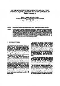
The input signal propagates through the network layer-bylayer. The signal-flow of such a network with two hidden layer is shown in Figure 1. Multi layer feed forward back propagation algorithm is used to train the network and tests the performance of the network. MLP networks are typically used in supervised learning problems. This means that there is a training set of input-output pairs and the network must learn to model the dependency between them. Multilayer Perceptron (MLP) network is a popular learning algorithm in a sense that neural network knows the desired output and adjusting of weight coefficients is done in such way, that the calculated and desired outputs are as close as possible. This paper is organized as follows. In next section, we introduce some related background including some basic concepts of back propagation algorithm with learning, training data set and testing data set determination and back propagation network generation using matlab toolbox. In the following section, we explain results and performance evaluation of multilayer perceptron (MLP) using back propagation algorithm. Finally, we have some conclusions with future work.
2 Overview of Back Propagation Algorithm 2.1 Back Propagation Algorithm Back propagation is a form of supervised learning for multilayer nets, also known as the generalized delta rule. Error data at the output layer is back propagated to earlier ones, allowing incoming weights to these layers to be updated. It is most often used as training algorithm in current neural network applications. The back propagation algorithm is an involved mathematical tool; however, execution of the training equations is based on iterative processes, and thus is easily implementable on a computer [7]. During the training session of the network, a pair of patterns is called input pattern and desired pattern. The input pattern causes output responses at each neurons in each layer and, hence, an output ok at the output layer. At the output layer, the difference between the actual and target outputs yields an error signal. This error signal depends on the values of the weights of the neurons in each layer [8]. This error is minimized, and during this process new values for the weights are obtained. The speed and accuracy of the learning process that is, the process of updating the weights-also depends on a factor, known as the learning rate. 271
IJSTR©2015 www.ijstr.org
INTERNATIONAL JOURNAL OF SCIENTIFIC & TECHNOLOGY RESEARCH VOLUME 4, ISSUE 02, FEBRUARY 2015
ISSN 2277-8616
If l=1 which means the j neuron is in the first hidden layer then we get,
Here,
is the jth element of the input vector x(n).
Let, L is the depth of network. If the neuron j is in the output layer that means l= L then
Fig. 1. Back Propagation Network. The process then starts by applying the first input pattern and the corresponding target output. The input causes a response to the neurons of the first layer, which in turn cause a response to the neurons of the next layer, and so on, until a response is obtained at the output layer. That response is then compared with the target response; and the difference (the error signal) is calculated. From the error difference at the output neurons, the algorithm computes the rate at which the error changes as the activity level of the neuron changes. So far, the calculations were computed forward (i.e., from the input layer to the output layer). Now, the algorithms steps back one layer before that output layer and recalculates the weights of the output layer (the weights between the last hidden layer and the neurons of the output layer) so that the output error is minimized [9]. The algorithm next calculates the error output at the last hidden layer and computes new values for its weights (the weights between the last and next-to-last hidden layers). The algorithm continues calculating the error and computing new weight values, moving layer by layer backward, toward the input. When the input is reached and the weights do not change, (i.e., when they have reached a steady state), then the algorithm selects the next pair of input-target patterns and repeats the process [10]. Although responses move in a forward direction, weights are calculated by moving backward. Hence the name of the algorithm is back-propagation.
2.2 Implementation of Back Propagation Algorithm The back-propagation algorithm consists of the following steps: 1. Initialization: At first the algorithm has to be initialized considering no prior information is known and picking the synaptic weights and thresholds from a uniform distribution. The type of activation function is sigmoid. 2. Presentations by Training Examples: The network has to be presented by epochs of training examples to perform forward and backward computations. 3. Forward Computation: Let us consider, the input vector to the layer of sensory nodes is x(n) and the desired response vector is d(n) which is in the output layer of computation nodes. In forward computation, the network’s local fields and function signals are computed by proceeding forward through the network by layer by layer basis. If sigmoid function is used, the output signal is obtained by the equation below:
So the error signal will be
Here, is the jth element of the vector of desired response d(n). 4. Backward Computation: In backward computation the local gradients of the network is calculated by the following equation [11]:
represents differentiation with respect to the argument. The synaptic weights of the network in layer l have to be adjusted according to the generalized data rule. If η is the training –rate parameter and α is the momentum constant, we get,
5. Iteration: Finally the forward and backward computations have to be iterated until the chosen stopping criterion is met. As the number of iterations increases the momentum and learning-rate parameters are adjusted by decreasing the values.
3 EXPERIMENT Our given image is RGB image. For our work, we first convert RGB image to gray scale image and then gray scale image to binary image. Step 1: Boundary Determination and Curve Fitting In this section, two classes of training data are determined and the boundary is set up. The goal of this task is and just is to 272
IJSTR©2015 www.ijstr.org
INTERNATIONAL JOURNAL OF SCIENTIFIC & TECHNOLOGY RESEARCH VOLUME 4, ISSUE 02, FEBRUARY 2015
ISSN 2277-8616
test and justify the classification accuracy of the given picture which is shown in figure 2. We divide the picture into two classes. The wooden part of the door with frame represents as Class 1 and rest of the picture is treated as Class 2.
Fig. 3. Image divided by colours ‘black’ and ‘white’.
Fig. 2. Given Picture. In order to classify these two classes clearly, twenty boundary lines are needed. The specific data coordinate point is obtained by using data cursor, which can be found in the MATLAB figure toolbar. The data cursor sets up the zero point (0, 0) inherently at the top left corner of the given picture. The (0, 0) point in the matlab simulation output of our project should be the bottom left corner. In order to produce the boundary lines effectively and efficiently, curve fitting is employed. Step 2: Training Data Set and Testing Data Set Determination After we have the boundaries of the wooden part of the door with frame, the next step is to obtain points from the original picture and sort the points by colour (black and white). First of all, 252353 points are obtained uniformly from the picture with a resolution of pixels. Then, all the points in the wooden part of the door with frame is set as ―0‖ and the colour is set as black. Similarly, all the rest points are set as ―1‖ and the colour is set as white. So after this procedure, a matrix is generated as the database for our test.
The first two columns represent the X co-ordinate and Y coordinate of a certain point. The third column of the matrix represents the colour of the certain point. For training data set we randomly select 7000 points from 252353 points. The testing data set has 2100 points that are selected from the whole picture randomly. Step 3: Simulation Results In this paper, we used multilayer perceptron to train the network with back-propagation algorithm. The number of hidden layer is two and the number of hidden neuron is 51 and 15 respectively. From the training window, we can access three plots: performance, training state, and regression. The performance plot shows the value of the performance function versus the iteration number. Each iteration of the complete training set is called an epoch. In each epoch the network adjusts the weights in the direction that reduces the error. As the iterative process of incremental adjustment continues, the weights gradually converge to the locally optimal set of values. Many epochs are usually required before training is completed. Training automatically stops when generalization stops improving, as indicated by an increase in the Mean Square Error (MSE) of the validation samples. The Mean Squared Error (MSE) is the average squared difference between outputs and targets. Lower values are better while zero means no error. Regression is used to validate the neural network and justify the relationship between the outputs of the 273
IJSTR©2015 www.ijstr.org
INTERNATIONAL JOURNAL OF SCIENTIFIC & TECHNOLOGY RESEARCH VOLUME 4, ISSUE 02, FEBRUARY 2015
network and the targets. Regression analysis is performed to measure the correlation between outputs and targets. If the training were perfect, the network outputs and the targets would be exactly equal, but the relationship is rarely perfect in practice. Table 1 The Mean Square Error (Mse) And Regression (R) Values For The Training, Validation And Testing Type of Data
MSE
R
Training Testing Validation
2.35e-2 2.2e-2 2.7e-2
0.94212 0.92733 0.92745
4
ISSN 2277-8616
CONCLUSION
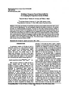
In this paper at first we studied the back propagation algorithm for training the multilayer artificial neural network. We used Back-Propagation learning algorithm to train the feed forward neural network to perform a given task based on LevenbergMarquardt algorithm and also we evaluated the performance of the trained network. From our learning curve we see that the validation and test curves are very similar. For avoiding over fitting we used early stopping method. The main goal of early stopping is to divide data into two sets, training and validation. Validation error is not a good estimate of the generalization error. That is why we used early stopping method so that training is stopped when the validation error starts to go up. We performed regression R analysis to measure the correlation between outputs and targets. We created a regression plot for validating the network which shows the relationship between the outputs of the network and the targets. It is observed that the value of R is closer to 1 indicating the accurate prediction. When the data set was trained in Levenberg – Marquardt algorithms the performance obtained was in 248 epochs. Levenberg – Marquardt algorithm (LM) is the most widely used optimization algorithm.
REFERENCES [1] Zhao, Zhizhong, et al. "Application and comparison of BP neural network algorithm in MATLAB." Measuring Technology and Mechatronics Automation (ICMTMA), 2010 International Conference on. Vol. 1. IEEE, 2010. [2] Alsmadi M. K. S., K. Omar, and S. A. Noah (2009), ―Back Propagation Algorithm: The Best Algorithm among the Multi-layer Perceptron Algorithm‖, International Journal of Computer Science and Network Security, pp. 378-383.
Fig. 4. The Learning Curve. The relationship is rarely perfect in practice. For this implementation, the data set is collected from the given picture and Levenberg-Marquardt back-propagation algorithm is used for training the network. The performance of the proposed network is trained with back-propagation algorithm using MATLAB R2013a which is shown in Figure 4. We ran the back- propagation algorithm 50 times and through the figure we can see that the best validation performance happens at epoch 248. From our obtained learning curve we can see that the validation and test curves are very similar so we can conclude that learning with back-propagation algorithm does not indicate any major problems with the training. If the test curve had increased significantly before the validation curve increased, then it is possible that some over fitting might have occurred. But in our case no over fitting is occurred. The Regression plot shows the perfect correlation between the outputs and the targets. The result for training, validation and testing samples is illustrated in Table 1. It is observed that the value of R is closest to 1 indicating the accurate relation between outputs and targets. For our network, the training data indicates a good fit. The validation and test results also show R values that greater than 0.9. The outputs from Matlab software are: Accuracy = 94% (classification) Iteration = 248
[3] Svozil, Daniel, Vladimir Kvasnicka, and Jir̂ í Pospichal . "Introduction to multi-layer feed-forward neural networks." Chemometrics and intelligent laboratory systems 39.1 (1997): 43-62. [4] Pinjare, S. L., and Arun Kumar. "Implementation of neural network back propagation training algorithm on FPGA." Int. J. Comput. Appl 52.6 (2012): 0975-8887. [5] Mutasem khalil Sari Alsmadi, Khairuddin Bin Omar and Shahrul Azman Noah (2009), ―Back Propagation Algorithm: The Best Algorithm among the Multi-layer Perceptron Algorithm‖, International Journal of Computer Science and Network Security, Vol.9, No.4, pp.378-383. [6] Norhamreeza Abdul Hamid and Nazir Mohd Nawi (2011), ―Accelerating Learning Performance of Back Propagation Algorithm by Using Adaptive Gain Together with Adaptive Momentum and Adaptive Learning Rate on Classification Problems‖, International Journal of Software Engineering and its Applications, Vol.5, No.4, pp.31-44. [7] Alsmadi M. K. S., K. Omar, and S. A. Noah (2009), ―Back Propagation Algorithm: The Best Algorithm among the Multi-layer Perceptron Algorithm‖, International Journal of Computer Science and Network Security, pp. 378-383. [8] Haykin, Simon. Neural Networks and Learning Machines, New Jersey: Pearson Prentice Hall, 2008. 274
IJSTR©2015 www.ijstr.org
INTERNATIONAL JOURNAL OF SCIENTIFIC & TECHNOLOGY RESEARCH VOLUME 4, ISSUE 02, FEBRUARY 2015
ISSN 2277-8616
[9] Pinjare, S. L., and Arun Kumar. "Implementation of neural network back propagation training algorithm on FPGA." Int. J. Comput. Appl 52.6 (2012): 0975-8887. [10] Sapna, S., A. Tamilarasi, and M. Pravin Kumar. "Backpropagation learning algorithm based on Levenberg Marquardt Algorithm." CS & IT-CSCP 2012 (2012): 393398. [11] Haykin, Simon. Neural Networks and Learning Machines, New Jersey: Pearson Prentice Hall, 2008.
275 IJSTR©2015 www.ijstr.org