An Alternative to Arithmetic Coding with Local ... - People.csail.mit.edu

An Alternative to Arithmetic Coding with Local Decodability Yevgeniy Dodis New York University

Mihai Pˇatra¸scu AT&T Labs

Mikkel Thorup AT&T Labs

January 20, 2010

Abstract We describe a simple, but powerful local encoding technique, implying two surprising results: 1. We show how to represent a vector of n values from Σ using dn log2 Σe bits, such that reading or writing any entry takes O(1) time. This demonstrates, for instance, an “equivalence” between decimal and binary computers, and has been a central toy problem in the field of succinct data structures. Previous solutions required space of n log2 Σ + n/ lgO(1) n bits for constant access. 2. Given a stream of n bits arriving online (for any n, not known in advance), we can output a prefix-free encoding that uses n + log2 n + O(lg lg n) bits. The encoding and decoding algorithms only require O(lg n) bits of memory, and run in constant time per word. This result is interesting in cryptographic applications, as prefix-free codes are the simplest counter-measure to extensions attacks on hash functions, message authentication codes and pseudorandom functions. Our result refutes a conjecture of [Maurer, Sj¨odin 2005] on the hardness of online prefix-free encodings.

1

Introduction

Suppose we want to represent a vector A[1 . . n], where each element comes from some finite alphabet Σ. The optimal space is dn log2 Σe bits, and it can be achieved by treating the vector as a big number between 0 and |Σ|n − 1, and converting this number to binary. Unfortunately, this encoding has very poor locality: (1) we cannot encode a stream of symbols with a low-memory algorithm; (2) we cannot read or write a single element A[i] faster than decoding the entire vector. Taking an information-theoretic view point, this naive encoding is generalized (and strengthened) by the well-known arithmetic codes. To encode n independently chosen symbols from some distribution D, arithmetic codes use n · H(D) + O(1) bits in expectation, where H(·) denotes binary entropy. The basic idea is to map the space of possible inputs A to the interval [0, 1]. To represent the first letter, [0, 1] is broken into |Σ| intervals, and each letter a ∈ Σ gets an interval of length pD (a). The process continues recursively, subdividing the interval corresponding to A[1] in order to represent A[2], etc. After the (tiny) interval corresponding to A has been identified, one simply outputs the shortest binary number inside it. The challenge is to implement this conceptual idea efficiently with bounded precision arithmetic. The ubiquitous implementation, due to Witten et al. [WNC87, MNW98], can perform encoding and decoding of a stream in O(1) time per bit, using O(lg n) space. It is instructive to briefly review this algorithm, as it highlights the inherently non-local nature of arithmetic codes. Imagine encoding a stream of symbols sequentially, and maintaining a subinterval 1

of [0, 1] that represents the data so far. Whenever the interval is fully contained in [0, 12 ], a zero bit can be output, and we can re-normalize [0, 12 ] 7→ [0, 1] to gain precision. Similarly, once the interval is in [ 12 , 1], a one bit is output and we map [ 12 , 1] 7→ [0, 1]. Alas, this is not enough to keep the required precision bounded, as the interval may become [ 21 − ε, 12 + ε] for exponentially small ε. The trick of [WNC87, MNW98] is to re-normalize [ 14 , 34 ] 7→ [0, 1] whenever the current interval is fully contained in [ 41 , 43 ]. Since the next bit is not known, the algorithm simply increments a counter of “outstanding bits.” When the interval finally gets below or above the middle point, a burst of zeros or ones is written. Abstractly, this demonstrates how the encoding of one particular character may depend non-trivially on many surrounding characters. In this work, we give an alternative to arithmetic coding, for a uniform distribution D on Σ, which retains optimal compression, but enjoys strong locality properties.

1.1

Representing a Vector

The field of succinct data structures is preoccupied with representing data in close to optimal space, while still supporting useful queries. Representing a vector to support reads and writes to individual entries is perhaps the most foundational problem in the field, and thus has been a toy problem of particular interest. The naive way of supporting local access is to encode each element separately using dlog2 Σe bits (cf. Hamming codes versus arithmetic codes). This has a redundancy of Ω(n) bits when Σ is not a power of two; for instance, it wastes around 0.68n bits for decimal digits, Σ = {0, 1, . . . , 9}. Standard techniques in succinct data structure, dating back to [Jac89], could achieve constant access time using n log2 Σ + O(n/ lg n) bits of space. More recently, Golynski et al. [GGG+ 07] proposed an encoding with O(n/ lg2 n) redundancy and constant access time. Pˇatra¸scu [Pˇ at08] showed how to use recursion in succinct encodings, and achieved query time O(t) with a redundancy of O(n/( lgtn )t ). Setting t = O(1), we get redundancy n/ lgO(1) n with constant query time. For a growing body of problems, we have strong redundancy lower bounds of Ω(n/t) [GM03], Ω(n/t2 ) [Gol09], or n/ lgO(t) n [PV10]. Combining this with the non-locality of known optimal encodings, one may conjecture that any representation of a vector will require some nontrivial trade-off between the redundancy and query time. In this paper, we show that this is not the case, and a surprising optimal result is possible: Theorem 1. On a Word RAM, one can represent a vector A[1 . . n] of elements from a finite alphabet Σ using dn log2 Σe bits, such that any element of the vector can be read or written in constant time. The data structure requires O(lg n) precomputed word constants. From a conceptual perspective, the statement that a binary computer can represent data in any radix with no penalty has an inherent appeal. From a theoretical perspective, our result forms a nice contrast with the lower bounds of [PV10]. An overwhelming majority of succinct data structures rely crucially on the so-called rank/select problem. But it is proved in [PV10] that the redundancy needs to be at least n/ lgO(t) n, essentially matching the upper bound [Pˇ at08]. Two scenarios are plausible: either (1) the use of rank/select is inherent, and we need stronger lower bound techniques that apply to a broader class of problems; or (2) one can surpass the rank/select barrier by alternative techniques. In this paper, we illustrate scenario (2) for a natural, central question. One can hope that this opens the door to further improvements. In particular, if one could design locally-decodable

2

arithmetic codes for a biased distribution D, one would immediately solve the dictionary problem (a.k.a. set membership) — perhaps the most important remaining open problem in this field. Further discussion. The model of computation throughout this paper is the Word RAM, which is meant to formalize what is possible in imperative programming languages. The memory allows random access, and is organized into words of w bits, where w = Ω(lg n) in order to allow indices and pointers. A standard set of unit-cost operations is specified (in this paper, we only require addition, multiplication, and division). In the (unrealistic but mathematically cleaner) bit-probe model, Viola [Vio09] has recently shown that, if the query is allowed t bit probes, the redundancy must be at least n/2O(t) . Our new result provides a matching upper bound: simply simulate the actions of a RAM with t-bit words. It is unclear whether the abstract vector-representation problem has direct applications in practice. Applications to compressed Bloom filters are suggested by [Mit02]. In addition, extreme compression is of interest in current database applications. In many databases, columns have few common possibilities (as few as 3-5), so they can be compressed to an alphabet with these possibilities plus a letter indicating “other.” After pruning many rows using indexes, database queries degenerate into linear scans over ranges, and such scans are often memory-bound. Thus, it is worth using a (slightly) more CPU intensive algorithm for tighter compression of the records. In this context, not wasting one bit for small fields might be valuable. We mention that algorithms that exploit packing small fields into bits are currently deployed in a large commercial database [RS06, HRSD07]; in fact, this was the initial motivation behind our theoretical investigation.

1.2

Online Prefix-Free Encoding

Suppose one is to represent some n bits of information using a prefix-free code, where n is not fixed (i.e. it should be implicitly included in the code). In information theory, this task is known as universal coding, whereas in Computer Science, the term “prefix-free” is more often used (ambiguously). The term “self-delimiting code” is also in use. The textbook solution to this problem is given by Elias codes. For example, to encode a vector of n bits using the Elias delta-code, one can write: (1) as many zeros as there are bits in lg n, followed by a one; (2) the number n written in binary, using as many bits as indicated in part 1; (3) the n bits of data. This achieves n + O(lg n) bits, for any n. Applying this idea recursively, one obtains the Elias omega-code, which represents n input bits using n + log2 n + log2 log2 n + · · · + O(log? n) output bits. This bound is optimal. Prefix-free encodings are essential for communicating or storing any type of data, except fixedsize records. Less obviously, prefix-free encodings are often essential to ensure security of iterative constructions in cryptography, such as CBC-MAC [BRK94] and cascade constructions [GGM86, BCK96a, CDMP05, MS05]. In particular, prefix-freeness gives the simplest provably-secure countermeasure to various forms of extension attacks on hash functions, message authentication codes and pseudorandom functions, as discussed in Appendix A. In many natural applications, including those in cryptography, the message comes online, as a stream of bits, and the length of the stream is not known in advance. Elias codes are unusable in this setting. Instead, one wishes to design a simple code that can be encoded and decoded in one pass by algorithms maintaining small state (ideally, O(lg n) bits), and using lower overhead (ideally, O(1) time per input word).

3

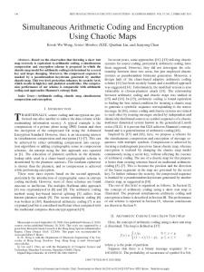
In practice, one typically assumes that the input comes in large blocks, say, b = 128 bits; the last block may be padded if it is incomplete. Then, one can append one bit after each block, indicating whether we have reached the end of file. With b = 128, this code has an overhead of almost 1%, which is acceptable, but a fairly steep price to pay just for encoding the length of the stream. More problematically, many cryptographic standards include work-arounds that eliminate the need for prefix-freeness, creating theoretical and practical burdens. In theory, the naive block-based solution gives a linear trade-off between redundancy and the space of the algorithm, by buffering S bits of input, and including an end-of-file marker before each block. Maurer and Sj¨ odin [MS05] conjectured that a linear redundancy might be necessary for smallspace online prefix-free encoding. This would explain why cryptographic standards tend to use ad hoc solutions instead, since a proportional increase in the stream size is unacceptable. Fortunately, we disprove this conjecture, by constructing a simple prefix-free code with ideal space and running time. As the first step, we point out the fallacy in the linear trade-off between space and redundancy: thinking in terms of integral bits. Let us imagine that we know n ≤ 2k . We can group blocks of k bits together, obtaining letters from an alphabet of [2k ]. We can then augment this alphabet with an endof-file symbol, eof. This introduces a redundancy of log2 (2k + 1) − log2 (2k ) = log2 (1 + 21k ) = O( 21k ) per block of data. This fractional waste aggregates to just O( nk /2k ) = o(1) bits overall. Thus, if one can efficiently move from base 2k to base 2k + 1 by an online algorithm, this refutes the conjecture of [MS05], and gives a prefix-free encoding using n + O(lg n) bits. In fact, using arithmetic coding already gives a result of this form, subject to the usual limitations of arithmetic coding (bursty output due to non-locality, and a running time is O(1) per bit). To be independent of n (we assumed we know k ≈ lg n), one can use a standard trick of “guessing” n up to a factor of two. By our techniques, we obtain two solutions to online prefix-free encoding with better properties. The first algorithm, described in Section 2 has the benefit of extreme simplicity, and fast running time (constant per word of input). We expect this to be the method of choice in practical implementations. The encoding also has excellent local properties: we can decode or modify a block by reading/writing only at O(1) code blocks. In addition, we can append to the stream or delete blocks from the end in O(1) time. The second algorithm, described in Section 5, has the benefit of better theoretical upper bounds, matching the optimal Elias bound up to O(lg lg n). We obtain: Theorem 2. There exists a universal code mapping n bits to n + log2 n + O(lg lg n) bits, which can be encoded and decoded by algorithms that use O(lg n) bits of space and take O(1) time per operation. Applications to Cryptography. As we already mentioned, prefix-free encodings (PFEs) are also essential for proving security of many natural cryptographic constructions which need to process variable-length messages. We will give many popular examples in Appendix A, but start with explaining the general reason why PFEs are useful in this context. In all such constructions, one first designs a “secure” compression function f : {0, 1}s × {0, 1}b → {0, 1}s , where b is called the block-length, and s is called the buffer-length. (Depending on the application, such f could be keyed or unkeyed, as we survey in Appendix A.) Intuitively, though, f allows one to securely process short, b-bit messages: given an initial buffer IV ∈ {0, 1}s (which could be a key or a fixed 4

m1 IV

m2 f

mn

...

f

f

y

Figure 1: The Cascade Mode of Operation Cascade(M, f, IV ). constant), the hash of m ∈ {0, 1}b is simply y = f (IV, m). Then, to process an arbitrarily long message M , one first splits M into b-bits blocks m1 . . . mn (so n ≈ |M |/b),1 and then iteratively process M via the cascade mode-of-operation, parameterized by the compression function f and the initialization vector IV ∈ {0, 1}s (see Figure 1): Cascade(M, f, IV ): Split M into b-bit blocks m1 . . . mn , where mi ∈ {0, 1}b and n = d|M |/be; Set x0 = IV ; For i = 1 to n Set xi = f (xi−1 , mi ); Output xn ; Typically, one can prove the following result: if the compression function f is “secure” and M is encoded in prefix-free form, then Cascade(M, f, IV ) is “secure” (where IV is either a cryptographic key or a constant, depending on the application). Intuitively, one can imagine building 2b -ary tree T , whose root is labeled by the IV , and each internal node m1 . . . mn at “depth” n is labeled by Cascade(m1 . . . mn , f, IV ). Typically, f is designed in a way that its ancestordescendant node pairs might be related in a “meaningful way” (e.g., Cascade(M M 0 , f, IV ) = Cascade(M 0 , f, Cascade(M, f, IV ))), while all other pairs of nodes are not related. Thus, if no two messages M1 and M2 are in the ancestor-descendant relationship, then the construction is secure. But this precisely corresponds to the fact that the messages are encoded in a prefix-free way. Moreover, in all known examples (see Appendix A), one can actually break the security of the construction if the PFE constraint is not enforced. Such attacks are typically referred to as extension attacks. Of course, if efficient one-line PFEs were known, one can easily prevent extension attacks using an on-line PFE. Unfortunately, since prior to our work it was believed (and explicitly conjectured by [MS05]) that one-line PFE comes at a significant cost, extension attacks are typically handled using various ad-hoc methods, different for each specific application. Specific examples are discussed in Appendix A, and include CBC-MAC [BRK94], cascade pseudorandom functions [BCK96a], Merkle-Damgard hash functions [CDMP05], domain extension of message authentication codes [MS05] and multi-property preservation [BR06, BR07]. In each of these examples, applying the cascade transform to the prefix-free encoding of the message gives the simplest-to-understand domain extension for the given cryptographic application. Thus, one 1

We will assume that |M | is a multiple of b. If not, one can always pad M with 1 followed by several (at most (b − 1)) zeros to make the last block mn full. Hence, w.l.o.g. we assume M ∈ ({0, 1}b )∗ .

5

Block number Input alphabet With eof Pass 1 Regroup Pass 2

1 B B+1 B B B

2 B B+1 B+3 B+3 B

3 B B+1 B−3 B−3 B

4 B B+1 B+6 B+6 B

5 B B+1 B−6 B−6 B

6 B B+1 B+9 B+9 B

... ... ... ... ... ...

Figure 2: Implementing Short-Odd Long-Even (SOLE) Encodings. application of our results is that previously used ad hoc methods might not be necessary in these applications.

1.3

Organization

In Section 2, we begin by describing a very simple algorithm for prefix-free encoding in the streaming model. This algorithm assumes that the input comes in blocks of b ≥ 2 lg n + 2 bits, and outputs a code of n + 2b bits. While restrictive, this scenario is of interest in cryptography, where common message authentication schemes work with at least 128 bits at a time. The algorithm is very simple, and we expect it to be the practical choice for these application. Using the intuition from this algorithm, we formulate a general concept (information carriers) in Section 3. Used appropriately, this construct implies an optimal data structure for representing a vector (Section 4), and an online prefix-free encoding of size n + lg n + O(lg lg n) (Section 5).

2

SOLE Encodings

We assume the input stream consists of blocks of b ≥ 2 lg n+2 bits. This is relevant in cryptographic applications, where b = 128 or higher. We observe that this is very weak and reasonable information about n. The block length b = 128 is chosen this large, in part, because long streams are anticipated. Thus, the assumption is in the same spirit as working with a word length assumed to have at least lg n bits, so that pointers can be represented for whatever n happens to be. Let B = 2b be the alphabet of a block. Adding a special end-of-file symbol (eof), we obtain an alphabet of size B + 1. Our goal is to encode n + 1 letters from this alphabet (including the final eof) using n + 2 blocks of b bits. Observe that n + 2 blocks is optimal (if we measure space in multiples of blocks), since going from alphabet B + 1 to alphabet B must have some loss. The algorithm is best illustrated by Figure 2. Intuitively, it is simplest to view the algorithm as two separate passes through the stream. In Pass 1, we consider pairs of elements on positions (2i+1, 2i+2), for i ≥ 0. Grouped together,   2 the elements  form a number in range  (B + 1) . We decompose this number into two values: one in range B − 3i , and one in range B + 3i + 3 . The smaller range is placed on odd positions, while the larger one on even positions, hence the name “Short-Odd Long-Even (SOLE) Encoding.” The decomposition is simply a division by B − 3i, keeping the remainder and the quotient. The transformation is valid as long as: (B + 1)2 ≤ (B − 3i)(B + 3i + 3) ⇒ B ≥ 1 + 9i(i + 1) ⇒ n ≤

6

2 3

· 2b/2

Block number Input alphabet With eof Pass 1 Regroup Pass 2

1 B B+1 B+1 B+1 B

2 B B+1 B−1 B−1 B

3 B B+1 B+4 B+4 B

4 B B+1 B−4 B−4 B

5 B B+1 B+7 B+7 B

6 B B+1 B−7 B−7 B

... ... ... ... ... ...

Figure 3: Implementing Long-Odd Short-Even (LOSE) encodings. In Pass 2, we regroup the considering  elements,    pairs on positions (2i, 2i + 1) for i ≥ 1. These elements come from range B + 3i and B − 3i , respectively. Since (B + 3i)(B − 3i) < B 2 , we can group them together as a number in range [B 2 ]. This uses a multiplication by B + 3i. We have obtained 2b bits (two blocks), which we output immediately. It is clear that these two conceptual passes can be implemented as a single pass in an online streaming algorithm. We simply need to remember the state of each path (at most two integers each). The decoding algorithm is the straightforward inversion of this process, implementing Figure 2 bottom-up. We stress the interesting locality of our encoding. For instance, we can decode an arbitrary block by reading just 4 consecutive blocks of the code. Modifying a block similarly involves only 4 output blocks. Finally, we can decide to append to the stream or delete blocks from the end; both operations take O(1) time. Termination. An important component of the algorithm that we have not described is the termination behavior, once eof is received. We imagine that the encoding proceeds indefinitely, with an infinite stream of zeros following eof. When the decoding algorithm has decoded the eof symbol, it stops immediately. Thus, in the encoding, it suffices to stop as soon as the eof symbol has been completely output. Trivially, this requires at most two zeros after eof, but in fact the encoding turns out to have only one additional block by a more careful analysis.   If eof appears on an even position (say, 2i), the final element after Pass 1 is in range B + 3i .   Combined with a zero value from range B − 2i , Pass 2 outputs the final two blocks. If eof appears on an odd position (say, 2i + 1), Pass 1 processes an appended to  zero element  have a complete pair. The quotient computed in Pass 1, though theoretically in B + 3i + 3 , is in fact in {0, 1}, since the last element was a zero. This makes it to the output unchanged by Pass 2, since all subsequent values are zero. LOSE Encodings. An alternative scheme with almost identical properties is the Long-Odd Short-Even (LOSE) encoding. For completeness, this algorithm is sketched in Figure 3.

3

Information Carriers

Let us re-examine the behavior of SOLE encodings for intuition. After seeing 2n blocks, the algorithm has written 2n − 1 blocks to the output, and is left with a number in range B + 3n . In keeping with the terminology of [Pˇ at08], we shall call this number a spill.

7

x

y

s

m Figure 4: Lemma 3 implements the box depicted.   The algorithm proceeds by grabbing two more blocks, i.e. a number in (B + 1)2 . Its first worry is to complete the spill with some information, to obtain two full blocks of output. That B2 means that the spill must be combined with a value in range b B+3n c ≈ B − 3n.   To identify  some useful information in range B − 3n , the algorithm takes the new number in (B + 1)2 modulo B − 3n. The result is combined with the spill and immediately output. Remaining now is the quotient of the division, a number in range new spill. This motivates us to formulate the following general lemma:

(B+1)2 B−3n

≈ B + 3n + 3. This is the

Lemma 3. Let X, Y ≤ 2w . We can injectively map (x, y) ∈ [X] × [Y ] to (m, s) ∈ [2M ] × [S], with the following properties: √ • S is chosen as a function of X and Y , but S = O( X); • the map can be evaluated in O(1) time; • x can be decoded from m and s, in O(1) time; • y can be decoded from m alone, in O(1) time; • the redundancy of this encoding scheme is:  

M + log2 S − log2 X + log2 Y = O √1X . Think of the range [2M ] as M bits, and [S] as a spill. The lemma is best understood in terms of Figure 4. We have some value y that we want to store immediately. Unfortunately, the range |Y | is not a power of two, so we cannot simply write y to memory without losing entropy. Instead, we use some unrelated x as an information carrier: it only helps in committing y to memory. Proof. Say we will use M memory bits. The entire information about y must  be in these M bits. M In addition to y, the bits can store a quantity from the universe C = 2 /Y . The redundancy in doing this rounding is at most:   M       
2 1 Y 1 M R1 = M −log2 Y · ≤ M −log2 2 −Y = log2 = O =O . Y 1 − Y /2M 2M C Now x is broken into two components: a value in the universe [C], to be combined with y, and a spill of size S = dX/Ce. This decomposition introduces a redundancy of:        X X +C C R2 = log2 C + log2 − log2 X ≤ log2 ≤ O . C X X 8

√ Balancing the two redundancies, R1 = R2 , we find that we should set C = Θ( X) and obtain R1 = R2 = O( √1X ). The overall redundancy is, by the chain rule:

M + log2 S − log2 X + log2 Y =


M − log2 Y − log2 C + log2 C + log2 S − log2 X) = R1 + R2 .

Mapping (x, y) to (m, s) takes one division and one multiplication. (We assume here that X and Y are fixed, so constant like C are precomputed.) Extracting y from m takes one division, and extracting x from (m, s) takes one division and one multiplication. In practice, it is standard to replace any integer division by a constant with two multiplications (precomputing the multiplicative inverse to w bits of precision).

4 4.1

Representing a Vector A First Attempt

We now turn to the problem of representing a vector A[1 . . n] of elements from Σ, supporting local access. A direct approach is to simply iterate Lemma 3. Formally, we group O(logΣ n) consecutive elements into elements x1 , . . . , xN from a universe X = Θ(n2 ). Initially, we start with a null spill, Y0 = 0. Applying the lemma, we obtain some memory bits M0 (which we write to memory), and some spill Y1 . Then, we store the spill from Y1 by using x2 as the information carrier, and obtain a spill Y2 , etc. Observe √ that, while the spill size Yi may depend nontrivially on Yi−1 , our lemma guarantees that Yi = O( X), i.e. the spill universe doesn’t grow without bounds. √ The redundancy introduced in each step is O(1/ X) = O(1/n). Thus, the overall redundancy is O( N m ) = o(1), plus one bit at the end, when we simply write down the last spill. To prove this formally, note that our definition of redundancy admits a chain rule: X
X
e log2 Yn d+ Mi − n log2 Σ ≤ 1 + Mi + log2 Yi − log2 Yi−1 − N log2 X i

i

= 1+

X

Mi + log2 Yi − log2 Yi−1 − log2 X




≤ 1+N ·O



√1 X

i

To read an element A[i], we first calculate to which xj it belongs. Then, we recover the spill yj from the memory written in step j + 1. Finally, we recover xj from the spill yj and the memory written in step j. Updating an xj can be done by recomputing the actions of steps j and j + 1. Spill yj may change in the process, but this only affect the memory written in step j + 1, and does not propagate to yj+1 . Unfortunately, this approach requires N = O(n/ lg n) precomputed constants. Indeed, each Yj is distinct, and even the number of bits written to memory in each step varies. This was not a problem in the SOLE encoding, as X = 2b + 1, so the Yj values could be approximated by an arithmetic progression. Here, X can be far from a power of two, and the behavior of the Yj ’s can be rather irregular inside a universe of O(n).

4.2

A Tree Representation

To reduce the number of precomputed constants to O(lg n), we will use a tree structure. As before, we group elements into N values from universe X = Θ(n2 ). Group these values into a binary tree,

9



as in the standard representation of a heap. This is an implicit representation, i.e. we simply define 2i and 2i + 1 as the children of node i, and bi/2c as the parent of node i. Each node will receive two spills, one from each child. It will combine these into a single value yi , and use its own value xi ∈ [X] as the information carrier to store yi . The resulting new spill is propagated to the parent. Note that, even though spills are propagated up, there is no recursion happening at query time. To obtain a value stored in a node v, we go to v’s parent and obtain v’s spill from the parent’s memory bits. Then, we compute v’s value from the spill and its own memory bits. To update some xi , we simply reconstruct the encoding of node i and its parent. The advantage of the arboral representation is that all nodes on a level are handled using O(1) precomputed constants. We have three types of nodes on level dlog2 ne − k: • A prefix of the nodes have subtrees that are complete binary trees of height k. • Following this, at most one node has a subtree that is not complete. • The remaining nodes have subtrees that are complete binary trees of height k − 1. The nodes in each of these three classes, from a given level, have identical constants generated by Lemma 3, since the spills from the children are identical by induction. Therefore, for each class of nodes on each level, we need to remember the following information: • • • •

the the the the

number of nodes in this class; location of the memory bits from the first node in the class; spill sizes received from the two children; constants of Lemma 3.

The level of node i is blog2 ic. We note that this can be computed by O(1) Word RAM operations, as shown in [FW93]. Once the level is known, we can determine in constant time the class of the node, and retrieve the constants and memory locations necessary for decoding. The last bit. By the construction from above, the total redundancy introduced by the applications of Lemma 3 is o(1) bits. Up to one bit of redundancy is then lost by rounding when the final spill is stored. Thus, we use dn log2 Σ + o(1)e, which could be equal to dn log2 Σe + 1. As a theoretical amusement, we mention that the space can be reduced to the optimal dn log2 Σe+ 1. The idea is that the o(1) term can be made O(n−c ), for any constant c, if one uses arithmetic on O(c lg n)-bit integers. But results on linear forms in logarithms show [BW92] that n log2 Σ is bounded away from an integer by 1/nO(1) , for any constant Σ. Thus, setting c high enough will ensure that n log2 Σ + O(1/nc ) ≤ dn log2 Σe. (For instance, when Σ = {0, 1, 2}, it suffices to set c = 1, 179, 648.)

5

Prefix-Free Codes via Information Carriers

In this section, we show how to obtain online prefix-free codes of size n + lg n + O(lg lg n), getting exponentially closer to the Elias bound of n + lg n + lg lg n + . . . We view the input as partitioned into blocks of slowly growing size: after n bits have been seen, the next block consists of the subsequent 2dlog2 ne bits. Let N be the number of blocks; the N -th block may be incomplete. For the first N − 3 blocks, we proceed as follows (with a buffer of O(lg n) bits, one simulate the operations with a 3-block lag, effectively learning about the end of file 3 blocks in advance). Let the 10

size of the block be 2k. There are 22k possible values for the block, but we artificially enlarge this universe to X = 22k + 2k . The redundancy introduced is log2 (22k + 2k ) − log2 (22k ) = O(2−k ). To understand the total redundancy over all blocks, note that there are O(2k /k) blocks with a fixed value of k, so the total cost over them is O(1/k). Summing for k up to lg n, we obtain O(lg lg n) bits of redundancy. Now 3 sequentially to every block. The redundancy introduced at each stage is √ apply Lemma −k O(1/ X) = O(2 ). This is O(lg lg n) bits over all blocks, as shown above. When we reach block N −2, we signal the imminent end of file. Normally, a block is encoded only in the {0, . . . , 22k − 1} range of the universe [X]. For block N − 2, we use a value in {22k , . . . , X}, which indicates the end of file. The value used will encode only the first k bits of the block (remember that X = 22k + 2k ). The lost entropy is log2 X − log2 (2k ) = k + O(1) = log2 n + O(1). Now, we encode block N − 1 as if nothing has happened. This is necessary because the decoding algorithm only learns about the end of file with a delay of one block: seeing the end of file flag requires the spill after block N − 2, and this is only available after block N − 1 has been written. Finally, we output the spill after block N − 1 (wasting a bit for rounding), the k bits that we ignored in block N − 2, and block N . As block N has variable length (it may be incomplete), we use an Elias code, for a cost of O(lg k) = O(lg lg n) bits.

References [AB99]

Jee Hea An, Mihir Bellare, Constructing VIL-MACs from FIL-MACs: Message Authentication under Weakened Assumptions, CRYPTO 1999, pages 252-269.

[BW92]

Alan Baker and Gisbert W¨ ustholz. Logarithmic forms and group varieties. Journal f¨ ur die reine und angewandte Mathematik, 442:19–62, 1992.

[Bel06]

Mihir Bellare, New Proofs for NMAC and HMAC: Security without CollisionResistance, Advances in Cryptology - Crypto 2006 Proceedings, Springer-Verlag, 2006.

[BCK96a] Mihir Bellare, Ran Canetti, and Hugo Krawczyk, Pseudorandom Functions Re-visited: The Cascade Construction and Its Concrete Security, In Proc. 37th FOCS, pages 514523. IEEE, 1996. [BCK96b] Mihir Bellare, Ran Canetti, Hugo Krawczyk: Keying Hash Functions for Message Authentication. CRYPTO 1996: pp. 1–15. [BRK94]

Mihir Bellare, Joe Kilian, and Phillip Rogaway. The Security of Cipher Block Chaining. In Crypto ’94, pages 341–358, 1994. LNCS No. 839.

[BR06]

Mihir Bellare and Thomas Ristenpart, Multi-Property-Preserving Hash Domain Extension and the EMD Transform, In Advances in Cryptology - Asiacrypt 2006, pp. 299-314.

[BR07]

Mihir Bellare and Thomas Ristenpart, Hash Functions in the Dedicated-Key Setting: Design Choices and MPP Transforms, ICALP 2007, pp. 399-410.

[BR93]

Mihir Bellare and Phillip Rogaway. Random Oracles are Practical: A Paradigm for Designing Efficient Protocols. In Proceedings ACM Conference on Computer and Communications Security (1993), 62-73. 11

[CDMP05] Jean-Sebastian Coron, Yevgeniy Dodis, Cecile Malinaud and Prashant Puniya, MerkleDamg˚ ard Revisited: How to Construct a Hash Function, Advances in Cryptology, Crypto 2005 Proceedings: 430-448, Springer-Verlag, 2006. [FW93]

Michael L. Fredman and Dan E. Willard. Surpassing the information theoretic bound with fusion trees. Journal of Computer and System Sciences, 47(3):424–436, 1993. See also STOC’90.

[GGG+ 07] Alexander Golynski, Roberto Grossi, Ankur Gupta, Rajeev Raman, and S. Srinivasa Rao. On the size of succinct indices. In Proc. 15th European Symposium on Algorithms (ESA), pages 371–382, 2007. [GM03]

Anna G´ al and Peter Bro Miltersen. The cell probe complexity of succinct data structures. In Proc. 30th International Colloquium on Automata, Languages and Programming (ICALP), pages 332–344, 2003.

[GGM86]

Oded Goldreich, Shafi Goldwasser, and Silvio Micali. How to construct random functions. Journal of the ACM, 33(4):792–807, October 1986.

[Gol09]

Alexander Golynski. Cell probe lower bounds for succinct data structures. In Proc. 20th ACM/SIAM Symposium on Discrete Algorithms (SODA), pages 625–634, 2009.

[HRSD07] Allison L. Holloway, Vijayshankar Raman, Garret Swart, and David J. DeWitt. How to barter bits for chronons: compression and bandwidth trade offs for database scans. In Proc. ACM SIGMOD International Conference on Management of Data, pages 389– 400, 2007. [Jac89]

Guy Jacobson. Space-efficient static trees and graphs. In Proc. 30th IEEE Symposium on Foundations of Computer Science (FOCS), pages 549–554, 1989.

[Mit02]

Michael Mitzenmacher. Compressed Bloom filters. IEEE/ACM Transactions on Networking, 10(5):604–612, 2002. See also PODC’01.

[MNW98] Alistair Moffat, Radford M. Neal, and Ian H. Witten. Arithmetic coding revisited. ACM Transactions on Information Systems (TOIS), 16(3):256–294, 1998. See also DCC’95. [MS05]

Ueli M. Maurer and Johan Sj¨odin. Single-key AIL-MACs from any FIL-MAC. In Proc. 32nd International Colloquium on Automata, Languages and Programming (ICALP), pages 472–484, 2005.

[Pˇat08]

Mihai Pˇ atra¸scu. Succincter. In Proc. 49th IEEE Symposium on Foundations of Computer Science (FOCS), pages 305–313, 2008.

[PV10]

Mihai Pˇ atra¸scu and Emanuele Viola. Cell-probe lower bounds for succinct partial sums. In Proc. 21st ACM/SIAM Symposium on Discrete Algorithms (SODA), 2010.

[PR00]

Erez Petrank, Charles Rackoff, CBC MAC for Real-Time Data Sources, J. Cryptology 13(3): 315-338 (2000).

12

[RS06]

Vijayshankar Raman and Garret Swart. How to wring a table dry: Entropy compression of relations and querying of compressed relations. In Proc. 32nd International Conference on Very Large Data Bases (VLDB), pages 858–869, 2006.

[Vio09]

Emanuele Viola. Bit-probe lower bounds for succinct data structures. In Proc. 41st ACM Symposium on Theory of Computing (STOC), pages 475–482, 2009.

[WNC87]

Ian H. Witten, Radford M. Neal, and John G. Cleary. Arithmetic coding for data compression. Communications of the ACM, 30(6):520–540, 1987.

A

Applications to Cryptography

We now discuss several applications of prefix-free encodings (PFEs) in cryptography. As discussed in the the Introduction, all these applications could be viewed as processing the given n-block message M = (m1 , . . . , mn ) by the cascade mode of operation, parameterized by the appropriate compression function f : {0, 1}s × {0, 1}b → {0, 1}s and the initialization vector IV ∈ {0, 1}s . (Depending on the application, such f could be keyed or unkeyed, and the IV could be a key or a constant.) For completeness, we repeat this definition of the cascade mode below (see also Figure 1): Cascade(M, f, IV ): Split M into b-bit blocks m1 . . . mn , where mi ∈ {0, 1}b and n = d|M |/be; Set x0 = IV ; For i = 1 to n Set xi = f (xi−1 , mi ); Output xn ; CBC-MAC. The CBC-MAC is a very popular way to build a message authentication code (MAC) from a block cipher. Such block-cipher g can be viewed as a keyed permutation gk (m), where |m| = b, k is the secret key and m is the messages. The CBC-MAC of M is then defined by Cascade(M, fk , 0b ), where the compression function fk (x, m) = gk (x ⊕ m) is keyed and the buffer-length s = b. Namely, CBC-MAC(k, M ) = gk (mn ⊕ gk (mn−1 ⊕ . . . ⊕ gk (m2 ⊕ gk (m1 )) . . .)) It is well known that CBC-MAC is secure if the encoding M is prefix-free [BRK94]. In contrast, CBC-MAC is easy to break otherwise. For example, if y = CBC-MAC(k, m1 ) = gk (m1 ), then setting m2 = m1 + y, we get that CBC-MAC(k, m1 m2 ) = gk (m2 ⊕ y) = gk (m1 ) = y, meaning that it is easy to forge the MAC of (m1 , m2 ) after learning the MAC of m1 . The practical fix for the above problem (see [PR00]) is to use “encrypted CBC-MAC”: namely, have a fresh key k 0 in addition to k, and output gk0 (CBC-MAC(k, M )). Although this fix is quite simple, it doubles the size of the secret key, which could be undesirable for some applications. On the other hand, our method makes at most one more calls to the block cipher (due to adding two more blocks in our encoding), and also adds a little bit of complexity due to encoding and decoding procedure (which are simple, but nevertheless need to be done).

13

Cascade PRF. Another natural application of the cascade mode is to extend the domain of a pseudorandom function (PRF). Specifically, assume gk is a keyed PRF from b bits to s bits, where s is simultaneously the size of the key k and the output length of gk (m). Define the compression function f (x, m) = gx (m), and set the initial IV = k. Then the classical cascade construction is defined as Fk (M ) = Cascade(M, f, k). Namely, the cascade state xi keeps the current PRF key (initially equal to the actual key k), with each iteration using the next message block mi to set the new key xi to the the PRF of the message block mi under the old key xi−1 . We also remark that the classical GGM [GGM86] construction of a PRF Fk from a length-doubling pseudorandom generator (PRG) G : {0, 1}s → {0, 1}2s is also a special case of the cascade construction with b = 1. Indeed, the PRG G(k) = (G0 (k), G1 (k)) above, where |Gm (k)| = s and m ∈ {0, 1}, yields a 1-bit PRF gk (m) = Gm (k). It is well known [GGM86, BCK96a] that the cascade construction is a secure PRF of variablelength messages if and only if the messages are encoded in a prefix-free form. Intuitively, as long as any two message “diverge” at some point, the resulting key values become random and unrelated. In contrast, the extension attack is particularly simple and devastating. If M2 = M1 M 0 , then Fk (M2 ) = FFk (M1 ) (M 0 ), so one can easily compute the PRF of any “descendant” M2 from the PRF of the “ancestor” M1 , breaking the pseudorandomness of Fk . The clean fix is to use the NMAC variant [BCK96b, Bel06], where a fresh key k 0 is stored in addition to k, and one defines NMACk,k0 (M ) = gk0 (Gk (M )). Once again, although simple, this doubles the key size of our PRF. Hence, in practice an hoc variant of NMAC is used, called ˜ and essentially calls NMAC with k = HMAC [BCK96b, Bel06]. HMAC uses a single key k, 0 gc (k˜ + ipad) and k = gc (k˜ + opad), where c, ipad, opad are specific constants hardwired into the design of HMAC. This regains the short key size, but now the security analysis requires some ad hoc assumptions of our initial PRF g beyond the fact that is is a PRF. In contrast, using a PFE, one naturally regains a singe key k, has the same number of calls to gk , but adds a little bit of complexity due to on-line encoding/decoding, which is not needed in HMAC. Merkle-Damgard Hash Functions. The cascade mode of operation is the main technique for building cryptographic hash functions. Such a hash function H should take an arbitrary long message M = (m1 , . . . , mn ), and produce a short, s-bit hash value H(M ). the minimal requirement for such hash functions is collision-resistance: it should be hard to find M1 6= M2 such that H(M1 ) = H(M2 ). However, in many applications even stronger properties are needed from H: intuitively, a new value H(M ) should look random and independent from all previous values H(M 0 ) for M 0 6= M . This is formalized by modeling H as a random oracle [BR93]. Of course, in practice one uses concrete hash function H. In fact, practical hash functions, including the current standard SHA and the vast majority of other popular hash functions, precisely use the cascade mode of operations, applied to an appropriate compression function f .2 Specifically, H(M ) is defined precisely as Cascade(M, f, IV ), where f is a publicly known unkeyed hash function from (s + b) to s bits, and IV is a fixed constant. As observed by many papers, and formally addressed by Coron et al. [CDMP05], such design of H makes it very different from a “monolithic” random oracle, even if the compression function f is modeled as a fixed-length random oracle. In particular, the extension attack here is as follows: given y = H(M ) for any 2 Actually, one uses the so called strengthened Merkle-Damgard Transform, where the length of the message is appended as the last message block. However, this detail does not affect our discussion below, so we stick with “plain Merkle-Damgard”, which is precisely the cascade mode.

14

unknown value M , one can easily compute the value y 0 = H(M, M 0 ) = Cascade(M 0 , f, y), for any suffix M 0 . Clearly, this should not be possible if H was a true random oracle.3 Coron et al. [CDMP05] formally defined what it means to securely extend the domain of a random oracle, and gave four simple ways to provably circumvent extension (and all other generic) attacks. The cleanest solution is to simply encode the message in a PFE! However, prior to our work it was considered too wasteful. The second solution is to truncate a non-trivial fraction of the output bits. Unfortunately, this method suffers from relatively poor exact security (and, of course, gives shorter output). The third solution is similar in spirit to the NMAC PRF solution above, and requires an independent compression function f 0 . which is then applied to Cascade(M, f, IV ). Unfortunately, it is not practically convenient to design two different compression functions f and f 0 .4 Finally, the last method is similar to the HMAC PRF method above, and could be viewed as a specific ad hoc trick to avoid having two independent compression functions: it outputs Cascade(Cascade(0b M, f, IV ), f, IV ). Until our work, this was considered the method of choice, since only one compression function is used, the message can be processed on-line, and only two extra calls to f are made are made. With our on-line PFE, however, we end up making the same number of calls to f , but, arguably, obtain a result which is simpler to understand and explain (in terms of security). Domain Extension of MACs. Another natural usage of the cascade mode is to extend the domain of a message authentication code (MAC) fk : {0, 1}b+s → {0, 1}s . This is different from the CBC-MAC and the cascade-PRF applications above because the building block here is only assumed to be unpredictable, as opposed to pseudorandom (indeed, it is easy to see that the CBC-MAC and the cascade constructions are not always secure if the block cipher or the b-bit PRF are only assumed unpredictable [AB99]). Still, we can still define Cascade-MAC(k, M ) = Cascade(M, fk , 0s ), where our compression function fk is keyed by the same key k throughout (so called dedicated-key setting [BR07]). It was observed by Maurer and Sj¨ odin [MS05] that the Cascade-MAC is secure if M is encoded in a prefix-free form. (The extension attack here is a bit more complicated; we refer to [BR07].) On the other hand, without using on-line PFE (which was conjectured to be too wasteful by Maurer and Sj¨odin), several techniques to overcome this problem are known. The simplest one is to use, once again, an additional key k 0 , and apply fk0 to the output of the Cascade-MAC(k, M ) (see [MS05], which slightly optimizes the earlier suggestion of [AB99]). Without having two keys, several ad hoc solutions were developed by [MS05, BR07]. While offering comparable efficiency to using the basic cascade construction with our PFE, these solutions are arguably less intuitive than the basic cascade construction. We also notice that the dedicated key setting can also be used for the domain extension of PRFs, when fk is a assumed a PRF rather than a MAC (but one gets a PRF back as well). The discussion here is similar to the MAC case. 3

While this attack might appear theoretical, consider a simple PRF construction Fk (M ) = H(k, M ). It is clearly secure if H is a random oracle, but completely insecure (due to the extension attack above) when H is implemented by the cascade mode. 4 Ironically, one way to design two independent compression functions f0 and f1 from a single compression function f is to prepend 0 when calling f0 , and 1 — when calling f1 . However, this is equivalent to the classical “wasteful” PFE, where each but last block is prepended with 0, and the last block is prepended with 1. Clearly, our PFE will result in a much less wasteful solution.

15

Multi-Property Preservation. As we have seen, in all the application that we mentioned applying the PFE followed by the cascade construction works. Thus, the PFE followed by the cascade construction can be seen as a multi-property preserving (MPP) transform. As advocated by Bellare and Ristenpart [BR06, BR07], devising MPP transforms is advantageous in terms of reusing the existing implementations of hash functions, by designing compression functions which simultaneously satisfy several desired properties. However, since online PFEs were considered impractical, Bellare and Ristenpart [BR06, BR07] had to work relatively hard to design their MPPs. Arguably, the “PFE-then-Cascade” is is a much simpler MPP to understand and explain than the MPPs developed by [BR06, BR07]. Given that our work gives a very efficient PFE, our MPP also offers roughly the same efficiency than the MPPs of [BR06, BR07], so it could be an attractive alternative to those MPPs.

16