An Animated Multivariate Visualization for Physiological and Clinical Data in the ICU Patricia Ordóñez
Marie desJardins
Michael Lombardi
University of Maryland, Baltimore County 1000 Hilltop Circle, Dept. of CSEE Baltimore, MD USA
University of Maryland, Baltimore County 1000 Hilltop Circle, Dept. of CSEE Baltimore, MD USA
University of Maryland, Baltimore County 1000 Hilltop Circle, Dept. of CSEE Baltimore, MD USA
[email protected] [email protected] [email protected] Christoph U. Lehmann Jim Fackler Johns Hopkins School of Medicine 600 North Wolfe Street Baltimore, MD, USA 21287
[email protected]
Johns Hopkins School of Medicine 600 North Wolfe Street Baltimore, MD, USA 21287
[email protected]
ABSTRACT Current visualizations of electronic medical data in the Intensive Care Unit (ICU) consist of stacked univariate plots of variables over time and a tabular display of the current numeric values for the corresponding variables and occasionally an alarm limit. The value of information is dependent upon knowledge of historic values to determine a change in state. With the ability to acquire more historic information, providers need more sophisticated visualization tools to assist them in analyzing the data in a multivariate fashion over time. We present a multivariate time series visualization that is interactive and animated, and has proven to be as effective as current methods in the ICU for predicting an episode of acute hypotension in terms of accuracy, confidence, and efficiency with only 30-60 minutes of training.
Categories and Subject Descriptors J.3 [Life and Medical Sciences]: Medical Information Systems
General Terms Design
Keywords computational physiology, information visualization, multivariate, time series
Permission to make digital or hard copies of all or part of this work for personal or classroom use is granted without fee provided that copies are not made or distributed for profit or commercial advantage and that copies bear this notice and the full citation on the first page. To copy otherwise, to republish, to post on servers or to redistribute to lists, requires prior specific permission and/or a fee. IHI’10, November 11–12, 2010, Arlington, Virginia, USA. Copyright 2010 ACM 978-1-4503-0030-8/10/11 ...$10.00.
Figure 1: Tabular display of laboratory values of a neonatal intensive care unit (NICU) patient from Johns Hopkins Electronic Patient Record [5]. Occasionally, there is more than one entry per day.
1.
INTRODUCTION
Although the sophistication of methods to collect data in the ICU and the volume of data produced by them is greater now than at any point in the history of medicine, the information overload that providers face may inhibit the diagnostic process [4]. Providers are expected to examine large volumes of data and identify correlations between dozens to hundreds of parameters based on their own clinical experience in order to detect significant medical events. Yet, a psychological study in 2005 found that humans can only process up to four independent variables in bar graphs of statistical data accurately and efficiently. When a fifth variable was introduced, accuracy dropped to no better than random [3]. Existing visualizations of the data to assist providers in analyzing physiological and clinical data consist of a table as in Figure 1, or a plot of values for a particular parameter over time. The latter visualizations primarily focus on analyzing the data along multiple single dimensions, as in Figure 2. At times, the x-axis reflects an instance of a measurement instead of a point in time so that the measurements appear equally spaced in time, although they may in fact be dispersed irregularly, as seen in Figure 3. Because of parameter dependence and variation over time in a complex organism such as a human, examining the vital
Figure 2: Eclipsys SCC [2] display of a typical NICU patient. Note the scale of the y-axis is designed for adult values. Normal neonate systolic BP is 46-62 mmHg.
Figure 4: Lifelines visualization of a patient’s medical history
Figure 3: Example from unevenly spaced time intervals on the x-axis in Eclipsys SCC display [2].
signs and laboratory results in a multivariate temporal representation shows promise for providing greater insight into how the body and its vital organs function as a whole. We propose a multivariate visualization to assist providers in analyzing the large amounts of data in a multivariate fashion. This visualization not only captures the relationships between the variables, but also the rate of change of the variables over time because it is animated. Another motivation for this visual model is the need for personalization in medicine. The detection of an abnormal or unusual circumstance is typically based on the examination of the univariate parameters to identify values that fall above or below preset baselines and thresholds. These values are generally based on age, gender, and/or weight, and were established (often decades ago) by measuring these parameters in a large population of patients. While these values are appropriate for many people, they are not for others because of differences in lifestyle, genetic makeup, and environment. In the case of premature infants, while preset baselines and thresholds do exist, displays are adjusted to show the best display of adult data as seen in Figure 2 and thresholds are set to adult data. So how can a provider notice a decline or improvement in such cases? The answer is by comparing the infant’s current data against its previous data. Our visualization is designed so that an individual’s data is compared to itself for the purpose of detecting anomalies and recurring patterns.
2.
RELATED WORK
Current methods to visualize medical data from a multivariate perspective focus on visualizing multiple individual parameters over time by either stacking plots of several uni-
variate time series or overlaying them. The authors are not aware of other multivariate temporal visualizations designed for the bedside monitor to examine a patient’s clinical and physiological data in a multivariate fashion. Other existing medical visualizations for physiological and clinical data have focused instead on capturing a patient’s medical history. Visualizations of a patient’s medical history from a multivariate perspective have included Powsner and Tufte [12]. Their visualization created a series of scatterplots for each parameter. They also saw a need to visualize the average and the standard deviation for each parameter in their scatterplots as we do in our visualization. The Lifelines project by Plaisant et al. [11] created a visualization that was far more intuitive because it aligns each time line for a parameter to one time line. The time lines for the different parameters are stacked on top of one another and grouped into categories along the y-axis. The categories include Problems, Allergies, Diagnosis, Complaints, Lab-path, Imaging, Medications, Immunology, and Communication. When one category is expanded, ticks and lines are used to represent the events in the particular category such as the amount and type of medication administered at a given instance in time, as seen in Figure 4. Clicking on an event will render more detailed information about the event. Whereas Lifelines is an excellent visualization to represent a patient’s medical history for several months to years, it is intended for historical purposes with longer time scales than ours. Our visualization is aiming to create multivariate visual patterns in the display of a patient’s data over several hours that would alert a provider of an impending critical state. The KNAVE-II prototype developed by Shahar et al. [13] also examines a patient’s history over several months to years. The visualization is similar to Lifelines in that it contains stacked views of the different states, as seen in Figure 5. In contrast to the Lifelines project, it attempts to retrieve clinically significant domain-specific temporal abstractions from the data using multiple univariate time series. Other characteristics that make it different from Lifelines are that it examines the state of several vital organs such as the liver,
3.
Figure 5: KNAVE II visualization of a patient’s medical history
PRIOR WORK
Previously, we presented a paper where the primary objective of the visualization was to alert providers of a crisis in a pediatric intensive care unit patient with renal or respiratory failure. We created the Multivariate Time Series Amalgam (MTSA) [10] to represent the state of a patient, which was the first step in creating the current visualization. We used overlaid star plots [1] to represent the changing states of a patient over time. The visualization was personalized as described below in the Personalized View, but was static. Temporal changes were indicated by the color of the starplots, with the lighter colors representing earlier data and the darker ones representing the most recent data. The current visualization is dramatically improved through the addition of animation, which utilizes the human eye’s ability to detect motion and translate the motion into a direction. Thus, it is able to emphasize the rate at which a patient’s state changes over time, which is more medically significant than displaying that a change has occurred. It also captures the relationships between the parameters more effectively than the static version. Furthermore, we have added two additional views of the data: the Standard View and the Customized View.
4.
THE VISUALIZATION
The primary goals of the visualization were to alert providers of a crisis within a patient without the use of preset thresholds and to allow providers to efficiently examine changes in a patient’s state over time in a multivariate fashion. We decided to use a star plot [1] to achieve these objectives because star plots have the capability of representing multiple variables over time in a small area. The challenges included the handling of fragmented data, determining where to examine the data, and producing a multivariate time-series representation that providers would find medically significant.
4.1
Figure 6: Zoom Star visualization of 8 stocks over 3 weeks pancreas, and kidney as well as the state of other parameters. The states are customizable depending on what the provider is looking for in a patient. Again, this visualization is intended for examination of a patient’s historical data over several months to years, but like our visualization, it groups parameters according to their effect on vital organs. The most similar visualization that has been created for multivariate time series data is the Zoom Star [9]. Zoom Star overlays star plots in a 2D space with different colors and levels of transparency, but does not include the temporal granularity that ours does, nor is it animated. Zoom Stars are intended for categorical or quantitative data. In the case of quantitative data, it plots the limits of the intervals, as seen in Figure 6; in the case of categorical data, it plots dots along an axis where the diameter of the dot is proportional to the frequency of the category. Our visualization plots an approximation of time series data and emphasizes the change in the relationships between the variables over time.
Preprocessing Data
The quality of medical data is far from ideal because there are so many human factors that influence the measurement and documentation of the data. Therefore, significant effort is required to preprocess the data. In the case of the ICU data used for this paper, we used the validated clinical values, which were taken approximately every hour. Some of the parameter values contained missing data, meaning that the measurement was not taken at its designated time. These data points were linearly interpolated in order for all variables to have a value within the selected interval of 15, 30 or 60 minutes for the display. Although better techniques exist for interpolating the missing values, creating a visualization was the primary concern. Prior to rendering the visualization, a uniform scale for displaying the data had to be calculated on every axis for all parameters. In an effort to accomplish this task, we modified the concept of Piecewise Aggregate Approximation (PAA) that Eammon Keogh and Jessica Lin use for Symbolic Aggregate Approximation (SAX) [6]. PAA takes a univariate time series, divides it into equal sized intervals, and then approximates the value for each interval by averaging the values in the interval. We then created an MTSA [10] by interleaving the values of all the parameters for a given interval in a consistent order. The parameters are ordered according to their effect
Figure 7: MTSA Visualization of 10 hours of data averaged in 15-minute intervals on one of four vital organs - the heart, liver, lung, and kidney - and then alphanumerically. An example of the category for some parameters can be seen in Table 1. Thus, an MTSA is a picture of a patient’s average state during an interval. The MTSA for each interval is then plotted as a star plot in the visualization to create a series of overlaid stars plots and represent the patient’s changing state over time. The color of each star plot is used to indicate the temporal changes in the MTSAs over time with the lightest color representing the earliest interval, and the darkest color the most recent interval.
4.2
The Personalized View
For the Personalized View, the values in the univariate time series for each parameter were normalized prior to constructing the MTSA so that the average was 0 and the standard deviation was 1 as seen in Figure 7. This view is referred to as the personalized view because the data is being compared to itself during the normalization process, addressing one of the visualization’s primary objectives. The dotted red circle represents the patient’s average value over the entire period of time. Each point represents the deviation of a value from the average for its parameter. Another objective of the visualization is to capture the relationships between the variables as well as the rate of change of the variables over time. By plotting the standard deviation of the values from the patient’s average, the relationships between the variables and the rate of change of the variables over time are exaggerated. For this reason, the minimum and maximum values for each parameter are displayed in square brackets next to the label for the axis.
Figure 8: Standard View of patient in Figure 7
Table 1: List of Physiological Parameters Parameter Category Heart Rate(HR)
heart
Respiratory Rate (RR) Systolic Blood Pressure (SBP) Diastolic Blood Pressure (DBP) CO2
kidney
Creatinine (crea) BUN
Figure 10: The dialog box for viewing or changing the target and range values for a parameter
Sodium (na) Bilirubin
liver
NH3 Respiratory Rate(RR)
lung
pCO2 White Blood Cell Count (WBC)
Other
Core Temperature Hematocrit (Hct)
target value for the patient as well as a range value which determines the scale on the axis for a parameter. The result is a visualization that is customized to the provider’s preferences. With electronic medical records, it will be possible in the future to personalized the target and range values to reflect the patient’s ‘normal’ state. In the Customized View in Figure 7, the target and range have been adjusted for the child and the provider can examine the patient’s data more easily. The yellow circle represents the patient’s normal baseline and the two red dotted circles indicate an acceptable upper and lower bound for the patient’s data.
4.5
Interactive Properties
An important property of the visualization is that it should be interactive. In other words, the provider should be able to change the information that is displayed with the click of a button, and she should be able to understand what each point represents. The interactive properties of the visualization are described in the following section.
4.5.1
Figure 9: Customized View of patient in Figure 7
4.3
The Standard View
The Standard View was developed as a result of providers wanting to view changes in a parameter relative to a baseline. The Standard View plots the values along each axis relative to a target value entered by the provider by clicking on the Show Targets button. The center point of the star plots becomes equivalent to 0 and the axes are scaled such that the red dotted circle represents the target value for all parameters. In Figure 8, it is easy to see how a child needs very different target values than an adult. The target value is displayed next to the label on the axis before the square bracket. Although providers enjoyed being able to view how much a parameter had changed, they had lost the granularity that the Personalized View offered. This request spawned the next view, the Customized view.
4.4
The Customized View
With the Customized View, providers have the option of entering parameter-specific scaling for each axis. By clicking on the Show Targets button, the provider can enter a
The Controller
The left panel is the main controller of the visualization. The user can select a patient ID, desired interval, and desired length of time for viewing the data. The user must press the View button to display the data. By default, one patient is selected to display the MTSAs for 600 minutes in 15-minute intervals. The available parameters for the patient are loaded into the window on the left. The user must select the parameters she wishes to examine and press the View button to render the MTSA Visualization. Figure 10 displays the dialog box that is rendered to view and/or change the target and range values for a patient in the Standard and Customized Views.
4.5.2
Bottom Panel
When the View button is pressed, the canvas renders the overlaid MTSAs in the center of the view, and the time slider in the right panel is adjusted to the length of the selected time and interval lengths. A dashed red concentric circle highlights the average zero value for each of the parameters. The MTSAs are rendered in shades of blue and black. The temporal relationship of the overlaid MTSAs is indicated by the hue of the lines. The darkest line represents the most current interval and the lightest represents the oldest one. By default, the time slider is at time zero which renders all the MTSAs of the same thickness. All the axes for parameters that measure the state of a particular vital organ are located adjacent to one another and are of the same color.
Figure 11: A dialog box with information about a point in the visualization
The user may also click in the checkboxes next to the organ names to highlight only the parameters associated with the particular organ. The bottom panel serves as a color key for the axes in the visualization. Each axis is colored according to the parameter’s correlation to one of four vital organs. All other parameters are grouped in a category named Other. By clicking on the buttons with the category names, the user can change the colors of the corresponding axes if desired.
4.5.3
Top Panel
The top panel displays the personal information of the patient. The top panel may only be adjusted by selecting a patient ID and clicking on the View button in the bottom left of the visualization.
4.5.4
Documentation via Point and Click
Edward Tufte write about the importance of making the smallest effective change and of documentation [14]. Thus, we have incorporated the ability for the user to see how a value was calculated and to see the values which lead the creation of a point within the visualization. By clicking on a point, a dialog box is rendered that displays how the value of the point was calculated for the different views as well as the values used to calculate the point as seen in Figure 11. The information includes the actual value of the point, the name of the parameter, the time of the interval, the normalized value, the customized range, and the method of calculation followed by the points that were used to calculate the point.
4.6
Animation
One of the primary objectives of the visualization is the display of change in a patient’s state through animation. Humans have developed as hunters and gatherers. Thus, the ability to detect motion, analyze direction and speed are highly developed and are utilized in this animation. In addition to seeing the values displayed, our visualization is multidimensional since direction of change and its speed carry additional valuable information. TThe controller for the animation is the time slider on the right side of the visualization. The time slider is adjusted each time a patient’s data is loaded. It will be the length of the total time divided by the the interval plus one for the zero value. The provider is able to visualize the changes of a patient’s state interactively by moving the time slider. Switching tick in the slider highlights the MTSA for the selected interval. The color for the highlighted MTSA remains the same, while the others turn gray, and the line of the highlighted MTSA is made thicker. For example, Figure 12 highlights the interval between minutes 135 and 150. By
Figure 12: Personalized View highlighting the interval between 135 and 150 minutes clicking on the Start button, the provider can observe the changes in state over time because the slider will move from zero to its maximum value in 100 ms time steps creating an animation. The provider can make the animation move slower or faster by increasing or decreasing the time between the steps respectively. The value is entered in the text field next to the Start button.
4.7
Progamming Language
Our visualization was implemented using Java version 6.0 using the Swing interface. The decision to use Java was based on the platform independence of the code. Because MTSAs are intended to run in real-time to combine values from several different sensors, it is important for the implementation to be as platform independent as possible.
5.
EVALUATION
We have completed a pilot study on the visualization and its three views: Personalized, Standard and Customized.
5.1
Methods
In the study, 14 internal medicine residents who were within 2-3 months of completing their first, second, or third year of residency at St. Agnes Hospital in Baltimore were presented with up to 10 hours of physiological data for 10 patients and were asked to predict whether the patient would experience an episode of acute hypotension (AHE) in the following hour. The data came from the 2009 PhysioNet Challenge [7]. This data was selected because it is multivariate, temporal data and was in the challenge to automate the prediction of episodes of acute hypotension. Residents were provided with the age and gender of the patient, and five parameters; diastolic blood pressure (DBP), heart rate (HR), mean arterial pressure (MAP), respiratory rate (RR), and systolic blood pressure (SBP). Each resident used the visualization for five patients and the univariate time series plots of variable vs. time with supporting table data for the remaining five. Each survey presented the patients in varying order, alternating between the examining one patient in the visualization and examining the next patient with the plots and tabular data. Prior to commencing the survey, residents received between 30-60 minutes of training in how to use the visualization and were presented with examples
of patients who would experience AHE in the following hour and those who would not.
5.2
Limitations
In the survey, each resident was asked to enter the time started and the time completed for each question. In some cases, the residents only entered the time started and completion time was calculated by taking the difference between starting times. In three cases, the residents did not understand the instructions and the completion times were not entered correctly. These values were ignored. Because the clock used in the survey only differentiated time to the minute, when a resident completed a task in less than one minute, it was counted as one minute. Each resdident was also asked to answer the question ”‘How confident are you about your answer?”’. They answered on a scale from 1 to 5, where 1 meant ”‘not at all”’ and 5 meant ”‘Extremely”’. In some cases, residents omitted an answer. In these cases, the question was ignored. In future evaluation, we aim to automate the measuring of time and include a video tutorial to ensure that residents completely understand the instructions and how the visualization works. All residents who participated in the study were volunteers, thus explaining the small sample size. We are very grateful for their willingness to assist in the evaluation of the software. We are raising funds to be able to compensate participants in the future and hopefully increase the sample size.
5.3
Figure 13: Group 1 consisted of 8 residents. No verbal instructions or demonstrations were provided.
Results
The study was conducted in two sessions. The first session consisted of eight residents, which will be referred to as Group 1. Each resident was given a packet that described the visualization and provided between 30-60 minutes of written training exercises prior to beginning the survey. Several residents from Group 1 indicted frustration about not understanding the task at hand and commented that a video tutorial of the visualization and description of the survey would have been helpful. The accuracy by patient for Group 1 can be seen in Figure 13. The second session consisted of 6 residents, which will referred to as Group 2. For Group 2, a 10-minute demonstration of the visualization and description of the survey was conducted prior to the written training exercises, and accuracy improved, as seen in Figure 14. Overall, the residents were 52% accurate using the visualization and 56% accurate using the traditional method. Group 1 had 45% accuracy with the visualization versus 50% with the tables and plots, whereas Group 2 had 60% and 63% accuracy respectively, demonstrating the need for a clearer explanation of the the study to participants. A paired t-test between the results from using the visualization and the results using the tables and plots indicates the the difference in accuracy was not statistically significant (p < 0.05) for either group. The difference in accuracy between Group 1 and Group 2 was also not statistically significant as indicated by a t-test. Although neither group did much better than random, considering the residents had only been trained to use the visualization for 30-60 minutes (versus 9 months for the tables and plots), the visualization displays tremendous potential for analyzing multivariate physiological data over time. Interestingly enough, thirteen of the twenty eight submissions for the PhysioNet Challenge in
Figure 14: Group 2 consisted of 6 residents and had a 10-minute demonstration of the visualization and a description of the survey.
Figure 15: Graph of time taken to answer questions in the survey in the order they were presented.
easier analysis and more comparable to the visualization and the way it was presented is confusing. DBP-> HR-> MAP-> RR-> SBP It does not make sense with one. Overall it is good but needs to be more customized by our brain. Because right now we only see tables since many years and we feel comfortable because it does not change in seconds. Five variables changes very fast in personalized term. It is difficult to keep track all of them at same time. Figure 16: Confidence levels of residents while answering questions in the order they were presented. 2009 correctly categorized all 10 patients, 9 correctly categorized 8 out of 10, and 5 matched the results of the Group 2 by correctly categorizing 6 out of 10 [8], reflecting the need for automated decision support systems in medicine. One major difference between the task for the Physionet Challenge and what we asked of our residents was that the residents were not aware of the total number of patients who were to enter into AHE. Examining the confidence levels of all the residents in Figure 16, it is evident that the residents’ confidence level with the visualization was comparable to that of the traditional methods. A paired t-test between the results from using the visualization and the results using the tables and plots indicates the the difference in confidence was not statistically significant for either group. Completion time improved with increase use as seen in Figure 15. However, a t-test was not performed because of the inaccuracies in the method used to measure time. The total completion time of the survey ranged from 11 to 21 minutes, excluding the training. Most promising was the positive feedback from the residents. Great idea, and gives us a sense that the pt is ’alive’, since his vital signs are changing. It makes me think how quickly pt. can deteriorate. The personalized view is much better because you can see the trend. In medicine,the trend is important to predict happened next. I think it is very easy to interpret. However, it takes some getting used to and understanding how it works. I liked the personalized setup for seeing a generalized trend of values. I liked the standard setup to see where the pt. values are compared to a target. The customized setup was best to quickly see whether a pt.’s values are above or below normal.”’ Other comments that were not so favorable are below. Table shows different parameters in different table which can be plotted on the same table for
6.
FUTURE WORK
Currently, the implementation of visualization is not in real time. We are working with static data and going from the first interval of the static record where all the parameters exist to the indicated number of minutes for the display. Ideally, we would like to see how the visualization performs in a dynamic environment with data that is constantly changing. We would like to use the data directly from a bedside monitor in order to lessen the effects of missing data. In the cases, where we have to fill in missing data, we aim to use the best known approximation technique for a given parameter. Second, we aim to make the interface interact with a database such that a patient’s personal information can be displayed. However, for the purposes of confidentiality, all patient information in this paper is fabricated except for the actual time series data. Third, with the development of electronic medical records, it is now possible to use a patient’s medical history to automate the personalization of a patient’s baselines and thresholds. The target value for the Standard and Customized views could be obtained from an electronic medical record which would enhance the visualization’s patient specificity. The default if no target value is entered would be the traditional baseline and thresholds of a parameter. Fourth, we would like to use the visualization in a clinical decision support system to extract patients from a database who have experienced medically similar events or have similar phenotypic profiles given a patient’s clinical and physiological data. Lastly, several improvements are in the pipeline such as placing the visualization in a NetBeans Framework. In doing so, we could create several views, based on the influence of parameters to an organ, for example. The axes in these views would be static so that providers can learn to visually identify temporal patterns in the data.
7.
CONCLUSION
We have presented a visualization of the clinical and physiological data that enables providers to examine a patient’s state over time in a multivariate fashion. The visualization is interactive and animated, and has proven to be as effective as current methods in the ICU for predicting an episode of acute hypotension in terms of accuracy, confidence, and efficiency with limited training. Through more training, the visualization shows potential for improving how quickly and accurately a medical condition like hypotension is recognized.
8.
ACKNOWLEDGEMENTS
The authors would like to thank Drs. Kwame Ntim and Sapna Kuehl and all the medical residents who participated in the survey for their assistance in evaluating the visualization. The authors would also like to thank the MIT Laboratory of Computational Physiology (LCP) for allowing us to use the 2009 Physionet Challenge data set as well as for providing information about the results. The developer would also like to thank Blazej Bulka for his suggestions on how to implement the visualization; Dr. Penny Rheingans and the entire Data Visualization course in the fall 2008 semester for their feedback on how to improve the visualization; Daniel J. Scott at LCP for his code review of the visualization; and Dr. Roger Mark of LCP for his insight into developing the additional views. This research was possible due to a National Science Foundation Graduate Research Fellowship.
9.
REFERENCES
[1] J. M. Chambers, W. S. Cleveland, B. Kliener, and P. A. Tukey. Graphical Methods for Data Analysis. Boston: Wadsworth International, Duxbury Press, 1983. [2] Eclipsys. Clinical information solutions for critical care. http://www.eclipsys.com/hospitals-clinicalsolutions-critical-care.htm, September 2010. [3] G. S. Halford, R. Baker, J. McCredden, and J. D. Bain. How many variables can humans process? Psycological Science, pages 70–76, 2005. [4] T. Heldt, B. Long, G. Verghese, P. Szolovits, and R. G. Mark. Integrating data, models, and reasoning in critical care. In Engineering in Medicine and Biology Society, pages 350–353, 2006. [5] JHMCIS. EPR - electronic patient record. http://dcs.jhmi.edu/epr/index.cfm, September 2010. [6] J. Lin, E. Keogh, and S. Lonardi. Visualizing and discovering non-trivial patterns in large time series databases. Information Visualization, 4:61–82, 2005. [7] M.I.T. Laboratory of Computational Physiology. Physionet challenge. http://physionet.org/challenge/2009/, 2009.
[8] G. Moody and L. Lehman. Predicting acute hypotensive episodes: The 10th annual physionet/computers in cardiology challenge. Computers in Cardiology, 2009. [9] M. Noirhomme-Fraiture. Visualization of large data sets: the zoom star solution. International Electronic Journal of Symbolic Data Analysis, 2002. [10] P. Ord´ on ˜ez, M. desJardins, C. Feltes, C. U. Lehmann, and J. Fackler. Visualizing multivariate time series data to detect specific medical conditions. In AMIA Annual Symposuim, pages 530–534, 2008. [11] C. Plaisant, R. Mushlin, A. Snyder, J. Li, D. Heller, and B. Shneiderman. Lifelines: Using visualization to enhance navigation and analysis of patient records. In AMIA Annual Symposuim, pages 76–80, 1998. [12] S. Powsner and E.R.Tufte. Graphical summary of patient status. Lancet, 344:386–389, 1994. [13] Y. Shahar, D. Goren-Bar, D. Boaz, and G. Tahan. KNAVE-II: A distributed architecture for interactive visualization and intelligent exploration of time-oriented clinical data. In Proc. Artificial Intelligence in Medicine, pages 115–35, 2006. [14] E. Tufte. Beautiful Evidence. Graphic Press, 2006.
APPENDIX A.
PREFERRED ALLOCATION OF REVIEWING EXPERTISE
Medicine, Information Visualization
B.
LIST OF TOPICS
• Display and visualization of medical data • Physiological modeling • Computational support for patient-centered and evidencebased care