Linköping Studies in Science and Technology Dissertations, No. 1191
Efficient Information Visualization of Multivariate and Time-Varying Data Jimmy Johansson
Department of Science and Technology Linköping University
Norrköping 2008
Efficient Information Visualization of Multivariate and Time-Varying Data c 2008 Jimmy Johansson Copyright
[email protected]
Printed by LiU-Tryck, Linköping 2008 ISBN 978-91-7393-878-5
ISSN 0345-7524
Abstract Data can be found everywhere, for example in the form of price, size, weight and colour of all products sold by a company, or as time series of daily observations of temperature, precipitation, wind and visibility from thousands of stations. Due to their size and complexity it is intrinsically hard to form a global overview and understanding of them. Information visualization aims at overcoming these difficulties by transforming data into representations that can be more easily interpreted. This thesis presents work on the development of methods to enable efficient information visualization of multivariate and time-varying data sets by conveying information in a clear and interpretable way, and in a reasonable time. The work presented is primarily based on a popular multivariate visualization technique called parallel coordinates but many of the methods can be generalized to apply to other information visualization techniques. A three-dimensional, multi-relational version of parallel coordinates is presented that enables a simultaneous analysis of all pairwise relationships between a single focus variable and all other variables included in the display. This approach permits a more rapid analysis of highly multivariate data sets. Through a number of user studies, the multi-relational parallel coordinates technique has been evaluated against standard, two-dimensional parallel coordinates and been found to better support a number of different types of task. High precision density maps and transfer functions are presented as a means to reveal structure in large data displayed in parallel coordinates. These two approaches make it possible to interactively analyse arbitrary regions in a parallel coordinates display without risking the loss of significant structure. Another focus of this thesis relates to the visualization of time-varying, multivariate data. This has been studied both in the specific application area of system identification using volumetric representations, as well as in the general case by the introduction of temporal parallel coordinates. The methods described in this thesis have all been implemented using modern computer graphics hardware which enables the display and manipulation of very large data sets in real time. A wide range of data sets, both synthetically generated and taken from real applications, have been used to test these methods. It is expected that, as long as the data have multivariate properties, they could be employed efficiently.
iii
Acknowledgements My first thanks goes to my supervisor Mikael Jern for introducing me to information visualization and for all the help along the way. My sincere thanks to my supervisor Matt Cooper for the humongous number of discussions, advice and proof-readings. Many thanks are also directed across the Atlantic Ocean to my former colleague and exroom mate, Patric Ljung, for great collaboration and many interesting discussions. The inspiring support from Mats Lind and Camilla Forsell throughout the evaluation of my work has been of invaluable help. Thanks as well to all of my colleagues and friends at NVIS/VITA whose support through all the ups and downs has been so very much appreciated. Special thanks to Karljohan Lundin Palmerius for getting me addicted to LATEX and providing user support and even the template this thesis has been based on. Finally, I would like to thank my loving fiancée, Anette, for always supporting me and for reminding me that there are so many things in life to appreciate.
♦
This work has partly been supported by the Swedish Foundation for Strategic Research, grant A3 02:116.
v
vi
Contents I
Context of the Work
1
Introduction 1.1 Multivariate Data . . . . . . . . . 1.2 Multivariate Data Representations 1.3 Parallel Coordinates . . . . . . . . 1.4 Evaluation . . . . . . . . . . . . . 1.5 Research Challenges . . . . . . . 1.6 Contributions . . . . . . . . . . .
2
II
3 . . . . . .
. . . . . .
. . . . . .
. . . . . .
. . . . . .
. . . . . .
. . . . . .
. . . . . .
. . . . . .
. . . . . .
. . . . . .
. . . . . .
. . . . . .
. . . . . .
. . . . . .
. . . . . .
. . . . . .
. . . . . .
. . . . . .
. . . . . .
. . . . . .
. . . . . .
. . . . . .
. . . . . .
. . . . . .
5 6 9 10 13 14 15
Visualization of Multivariate and Time-Varying Data 17 2.1 Approaches for Many Data Items . . . . . . . . . . . . . . . . . . . . . . . . . . 17 2.2 Approaches for Many Variables . . . . . . . . . . . . . . . . . . . . . . . . . . 19 2.3 Approaches for Long Time Periods . . . . . . . . . . . . . . . . . . . . . . . . . 20
Contributions
23
3
Multi-Relational Parallel Coordinates 25 3.1 Circular Axis Arrangement . . . . . . . . . . . . . . . . . . . . . . . . . . . . . 26 3.2 Task-Based Analysis . . . . . . . . . . . . . . . . . . . . . . . . . . . . . . . . 28 3.3 Determination of Acceptable Distortions of Patterns . . . . . . . . . . . . . . . . 30
4
Revealing Structure in Cluttered Representations 33 4.1 High Precision Density Maps . . . . . . . . . . . . . . . . . . . . . . . . . . . . 34 4.2 Graphics Hardware Limitations . . . . . . . . . . . . . . . . . . . . . . . . . . . 35
5
Representations of Time-Varying, Multivariate Data 5.1 Interactive Analysis of Time-Varying Systems . . 5.2 Temporal Parallel Coordinates . . . . . . . . . . 5.2.1 Representation of Temporal Changes . . 5.2.2 Analysis of Temporal Structures . . . . . vii
. . . .
. . . .
. . . .
. . . .
. . . .
. . . .
. . . .
. . . .
. . . .
. . . .
. . . .
. . . .
. . . .
. . . .
. . . .
. . . .
. . . .
37 37 39 40 43
viii 6
CONTENTS Conclusions 45 6.1 Summary of Contributions . . . . . . . . . . . . . . . . . . . . . . . . . . . . . 45 6.2 Conclusions . . . . . . . . . . . . . . . . . . . . . . . . . . . . . . . . . . . . . 46 6.3 Future Research . . . . . . . . . . . . . . . . . . . . . . . . . . . . . . . . . . . 46
Bibliography
III
Appended Papers
49
55
A 3-Dimensional Display for Clustered Multi-Relational Parallel Coordinates
57
B Task-Based Evaluation of Multi-Relational 3D and Standard 2D Parallel Coordinates
65
C Perceiving Patterns in Parallel Coordinates: Determining Thresholds for Identification of Relationships
79
D Revealing Structure within Clustered Parallel Coordinates Displays
99
E Revealing Structure in Visualizations of Dense 2D and 3D Parallel Coordinates
109
F Interactive Analysis of Time-Varying Systems Using Volume Graphics
127
G Depth Cues and Density in Temporal Parallel Coordinates
135
List of Publications Papers A–G are appended to this thesis and cited by their respective letter throughout. The other publications are listed in the bibliography and cited accordingly. A Jimmy Johansson, Matthew Cooper and Mikael Jern. 3-Dimensional Display for Clustered Multi-Relational Parallel Coordinates. In Proceedings of IEEE International Conference on Information Visualisation, IV05, pages 188–193. London, UK, 2005. B Camilla Forsell and Jimmy Johansson. Task-Based Evaluation of Multi-Relational 3D and Standard 2D Parallel Coordinates. In Proceedings of Visualization and Data Analysis, SPIE-IS&T Electronic Imaging, SPIE Vol.6495, 64950C-1–12. San Jose, California, USA, 2007. C Jimmy Johansson, Camilla Forsell, Mats Lind and Matthew Cooper. Perceiving Patterns in Parallel Coordinates: Determining Thresholds for Identification of Relationships. Information Visualization advance online publication; DOI: 10.1057/palgrave.ivs.9500166, 2008, Palgrave Macmillan. D Jimmy Johansson, Patric Ljung, Mikael Jern and Matthew Cooper. Revealing Structure within Clustered Parallel Coordinates Displays. In Proceedings of IEEE Symposium on Information Visualization 2005, pages 125–132. Minneapolis, MN, USA, 2005. E Jimmy Johansson, Patric Ljung, Mikael Jern and Matthew Cooper. Revealing Structure in Visualizations of Dense 2D and 3D Parallel Coordinates. Information Visualization, volume 5, issue 2, pages 125–136, 2006, Palgrave Macmillan. F Jimmy Johansson, David Lindgren, Matthew Cooper and Lennart Ljung. Interactive Analysis of Time-Varying Systems Using Volume Graphics. In Proceedings of IEEE Conference on Decision and Control, pages 5083–5087. Paradise Island, Bahamas, 2004. G Jimmy Johansson, Patric Ljung and Matthew Cooper. Depth Cues and Density in Temporal Parallel Coordinates. In Proceedings of Eurographics/IEEE VGTC Symposium on Visualization, 35–42. Norrköping, Sweden, 2007. H Sara Johansson, Mikael Jern and Jimmy Johansson. Interactive Quantification of Categorical Variables in Mixed Data Sets. To appear in Proceedings of IEEE International Conference on Information Visualisation, IV08. London, UK, 2008. 1
2
CONTENTS I Jimmy Johansson and Matthew Cooper. A Screen Space Quality Method for Data Abstraction. In Proceedings of Eurographics/IEEE VGTC Symposium on Visualization. Eindhoven, The Netherlands, 2008. J Mikael Jern, Sara Johansson, Jimmy Johansson and Johan Franzén. The GAV Toolkit for Multiple Linked Views. In Proceedings of IEEE International Conference on Coordinated & Multiple Views in Exploratory Visualization, pages 85–89. Zurich, Switzerland, 2007. K Daniel Ericson, Jimmy Johansson and Matthew Cooper. Visual Data Analysis using Tracked Statistical Measures within Parallel Coordinate Representations. In Proceedings of IEEE International Conference on Coordinated & Multiple Views in Exploratory Visualization, pages 42–53. London, UK, 2005. L Nina Feldt, Henrik Pettersson, Jimmy Johansson and Mikael Jern. Tailor-made Exploratory Visualization for Statistics Sweden. In Proceedings of IEEE International Conference on Coordinated & Multiple Views in Exploratory Visualization, pages 133–142. London, UK, 2005. M Jimmy Johansson, David Lindgren, Matthew Cooper and Lennart Ljung. Interactive Visualization as a Tool for Analysing Time-Varying and Non-Linear Systems. In Proceedings of the IFAC World Congress, pages Tu–E03–Tp/8. Prague, Czech Republic, 2005. N Jimmy Johansson, Patric Ljung, David Lindgren and Matthew Cooper. Interactive Poster: Interactive Visualization Approaches to the Analysis of System Identification Data. In Poster Proceedings Compendium, IEEE Symposium on Information Visualization 2004, pages 23–24. Austin, Texas, USA, 2004. O Jimmy Johansson, Mikael Jern, Robert Treloar and Mattias Jansson. Visual Analysis Based on Algorithmic Classification. In Proceedings of IEEE International Conference on Information Visualisation, IV03, pages 86–93. London, UK, 2003.
Part I Context of the Work
3
Chapter 1 Introduction Due to the rapid advances in computer technology more data are produced today than ever before, from statistical data gathering, automated measurements and simulations. While this allows access to more and higher resolution data, users have to deal with data having a large number of items, variables and time steps. Visualization is the process of forming a mental image and is often a valuable tool when analysing such large and complex data. Information visualization is a research area which centres around aiding users in their efforts to explain and explore data using advanced, interactive techniques. A key challenge here is to find new, intuitive representations and mappings of data that facilitate interactive exploration by users. This thesis describes a number of new techniques to perform efficient visualization of large, multivariate, time-varying data. These new techniques principally build on a well-known visualization technique called parallel coordinates that enables the representation of multivariate data in a two-dimensional display. Methods for improving standard, two-dimensional parallel coordinates, as well as new graphical representations, are presented and evaluated through controlled user experiments. Though the majority of the contributions are related to parallel coordinates, many of the proposed methods can be generalized to other information visualization techniques. The purpose of this chapter is to introduce the nature of the data and the problems associated with its visualization. This will make it apparent how the contributions of the work address these issues. The next section of this chapter discusses multivariate data and gives definitions used throughout this thesis. Section 1.2 gives an overview of common techniques for representation of multivariate data. Section 1.3 discusses parallel coordinates in detail. In section 1.4, common forms of evaluation with respect to information visualization are discussed. Finally, this chapter discusses some of the most important research challenges and outlines the main contributions of the publications included in this thesis. The remaining chapters include the following. Chapter 2 describes current research with respect to large multivariate and time varying data. Chapters 3, 4 and 5 present the main contributions of this thesis. The last chapter then presents a summary of the contributions together with conclusions and suggestions for future research. The rest of this thesis contains the appended publications. 5
CHAPTER 1. INTRODUCTION
6
Table 1.1: A multivariate data set with two data items representing two cars (rows), each consisting of four variables (columns). Horsepower 153 102
1.1
Doors 5 3
Weight 1865 1234
Country Sweden France
Multivariate Data
In this thesis, a multivariate data item, d, is defined as d = {d1 , d2 , . . . , dN }, where di is a scalar and N is the number of variables (N ≥ 2). A multivariate data set is then one comprising M data items, instances of d, where M ≥ 2. The values of M and N vary widely depending on the application area. An illustration of a multivariate data set containing only two data items can be seen in table 1.1. The items here are cars where each is represented by a number of variables (horsepower, doors, weight, and country) which describe different properties of the two cars. Representing a multivariate data set in this tabular way, such that a data item (or simply an item) corresponds to a row and each variable corresponds to a column, is common and the one used throughout this thesis. As seen in table 1.1 the variables of the cars are not of the same type. Horsepower and Weight are continuous while Doors and Country are discrete. The discrete variables can, in turn, be divided into ordinal (Doors) and categorical (Country). Categorical values are a special type of variable since no ordering or similarity metrics are, typically, defined for this type of data. Visualization of categorical data is a research area in itself and is not studied in this thesis. The example data set illustrated in table 1.1 shows a data set which consists of values obtained at a specific point in time. A multivariate data set may also be time-varying, meaning that the data changes with time. In the case of a time-varying, multivariate data set, a requirement is that there should be at least one multivariate data item at each of a number of time steps. When analysing multivariate data, a range of features such as correlations, trends, clusters, and outliers are of interest to study. A number of examples are presented using two-dimensional scatter plots in figure 1.1. For a data set containing cars, for example, it might be of interest to find the relationship, if any, between how much a car weighs and its horsepower. Figure 1.2a shows a scatter plot representation of these variables. Another example could be, instead, that it is of interest to study the price of a single car over a number of years, as illustrated by the line graph in figure 1.2b. A final example could be to study differences in price for different makes of cars, see the bar chart representation in figure 1.2c. When a multivariate data set contains many items with respect to the available display area for its graphical representation the image can become overcrowded resulting in visual clutter. A cluttered image often makes analysis difficult and can cause the analyst to miss important relationships in the data. Visual clutter in a scatter plot is shown in figure 1.3 where no apparent structure is visible. Visual clutter is often particularly severe in representations of time-varying data sets since the total number of data items increases with each additional time step, of which there are often a large number.
1.1. MULTIVARIATE DATA
7
(a) When two variables are positively correlated they increase or decrease together.
(b) If one variable increases when the other decreases the two variables are negatively correlated.
(c) Two clusters of items that can be separated in both variables.
(d) An outlier is an item that does not follow the general trend, as shown by the lone item.
Figure 1.1: Examples of common relationships between two variables displayed in scatter plots.
If a multivariate data set contains many variables, an analysis can become time-consuming since the number of possible comparisons between pairs of variables is N (N − 1)/2. For a data set with 10 variables this yields 45 different pairs and for only twice as many variables, 20, 190 different pairs. Besides investigating the relationships between pairs of variables it is often of interest to study relationships between many variables, something that obviously becomes more difficult as the total number of variables increases. In this thesis, a multivariate data set containing either too many data items or variables for a visualization to be efficiently carried out using a chosen technique, is referred to as being large. Depending on the application area, efficient can have different meanings. In general, representations that enable efficient information visualization are those which convey information about data in a clear and interpretable way, and in a reasonable time.
CHAPTER 1. INTRODUCTION
8
Weight
Price
Price
Horsepower (a)
Car make
Year (b)
(c)
Figure 1.2: (a) the relationship between the weight and horsepower is plotted for a number of cars. (b) the price of a specific car is studied over a number of years. (c) the price of a number of cars for a specific year is compared.
Figure 1.3: A scatter plot representation suffering from a high degree of visual clutter making an analysis impossible.
1.2. MULTIVARIATE DATA REPRESENTATIONS
1.2
9
Multivariate Data Representations
This section will give an overview of common techniques for visualization of multivariate data. Additional information with more technical details can be found in [HMS01, Spe07, WB97]. Dimensionality Reduction To facilitate analysis of multivariate data, dimensionality reduction can be employed to reduce the number of variables in the data set. This can be achieved in many ways and techniques such as principal component analysis or self-organizing maps, see [HTF01, HMS01, Koh97], are often used. Reducing the number of variables to two or three enables a much easier representation using standard scatter plots or line graphs. Scatter Plot Matrix A scatter plot matrix consists of a number of individual scatter plots. Constructing a matrix of N (N − 1)/2 scatter plots allows the representation of all pairwise relationships in the data, where N is the number of variables. Analysing relationships over a larger number of variables than two is possible but, as discussed in [SR06], this requires a user to combine information from many two-dimensional representations to form the mental image of the multi-dimensional space. The same principle as exemplified with the scatter plot matrix could, of course, also be used with other uni- or bivariate representations. Iconic Displays Iconic displays are a set of techniques used for data representation and can include one or several variables. The strategy is to map data values to different geometric properties such as size, shape, length or volume. This causes variations in the data to be reflected by variations in the icons. Hence, a user might use this for visually identifying similar multivariate data items by comparing the overall shape of the icons or to search for outliers by identifying icons that are substantially different from their neighbours. Besides geometric properties, other features such as colour, transparency or texture can be used to convey additional features in the data. Some examples of commonly used icons are star glyphs [SFGF72], stick figure icons [PG88] and Chernoff faces [Che73]. Pixel-Oriented Techniques Pixel-oriented techniques [Kei96] map data values to coloured pixels. For a data set having N variables the screen is partitioned into N sub-windows, one for each variable. Inside each window the data values are then arranged according to some sorting technique. The fact that only a single pixel is used for each value enables a simultaneous representation of hundreds of thousands of values. On the other hand, using only a single pixel for each value makes it difficult to see more complicated structures. Table Lens The table lens [RC94] is a technique for visualization of multivariate data in tables. The technique allows each column to be viewed as a histogram and enables several user interactions such as sorting and searching. It uses a focus + context approach to distort the view and so enables one or more focus regions.
CHAPTER 1. INTRODUCTION
10
d1 d4 d3 d2
d5
Figure 1.4: A single data item displayed in parallel coordinates.
Parallel Coordinates The parallel coordinates technique [Ins85, ID90] makes it possible to analyse multivariate data in a two-dimensional display. The variables of a data set are mapped to parallel axes and a multivariate data item is displayed as a polyline that intersects the axes at the values of the variables. Since many of the methods presented in this thesis are applied to parallel coordinates, a more detailed description of the technique is given in the following section.
1.3
Parallel Coordinates
The parallel coordinates technique was developed by Inselberg for representation of hyperdimensional geometry [Ins85]. In 1990, Wegman suggested parallel coordinates as a technique for analysis of multivariate data [Weg90], which is also how the technique is used in this thesis. Since 1990, many extensions have been described in the visualization research literature and parallel coordinates is, today, one of the most commonly used techniques. Applications of parallel coordinates exist in a wide range of fields such as statistics, chemistry, meteorology, biology, and finance. Many interesting examples are found in [FPJJ05, GCML06, BS04, Eds03, tCMR07, RWK+ 06]. In parallel coordinates, variables are represented on coordinate axes placed parallel and uniformly spaced. A multivariate data item is then represented as a series of points on the axes that are positioned at the coordinate values of the data item. Two points on two adjacent axes are then connected by a line segment. This results in a multivariate data item being represented in parallel coordinates as a polyline. A parallel coordinates representation of a data item consisting of five variables is illustrated in figure 1.4 where the item d = {d1 , d2 , d3 , d4 , d5 } is represented. The scaling of each individual axis typically ranges from the variable’s minimum value at the bottom to its maximum value at the top. Depending on the application, other types of scaling might, however, be more appropriate [AA01]. When displaying a complete data set containing many data items, different types of relationships between the variables become apparent in the parallel coordinates display. Figure 1.5 illustrates, using two variables, how a positive linear relationship, a negative linear relationship
1.3. PARALLEL COORDINATES A
11 B
A
B (a) A positive linear relationship.
A
B
A
B (b) A negative linear relationship.
A
B
A
B (c) Two clusters.
Figure 1.5: Parallel coordinates (left) and scatter plots (right) showing common features in data. The two-dimensional points in Cartesian coordinates map to lines in parallel coordinates.
CHAPTER 1. INTRODUCTION
12
and a clustering appear in parallel coordinates. For each feature, the corresponding scatter plot is also displayed. With a positive linear relationship (figure 1.5a), the lines do not cross between the axes, which they do when a negative linear relationship is present (figure 1.5b). It is easy to see in the parallel coordinates representation in figure 1.5c that the two clusters can be separated in both variables. Using this system of parallel coordinates it is a simple task to add more axes, thus enabling the analysis of relationships between many variables. A multi-axis parallel coordinates representation supports a wide range of analysis tasks. Figure 1.6 illustrates such a representation for a number of data items with five variables (A–E). The first task that is supported is analysis of relationships between items over all variables. This is illustrated by the two items that are highlighted in brown. It is immediately apparent that they share similar values for all the five variables in the data set. Looking at variables A through C it can be seen that there exist two different three-dimensional clusters: one cluster consisting of the four items with the highest values at those variables and another consisting of the four items with the lowest values. Furthermore, since the lines cross between variables D and E, it is known that they have an approximately linear negative relationship. Variables A and B can, on the other hand, be identified as having a positive linear relationship. The task of identifying outliers is also supported, one example being the strong outlier in the relationship between C and D. The outlier is shown by the line going from the highest value on C (top of the axis) to the lowest value on D (bottom of the axis). This is a quite different behaviour compared with the other lines that seem to fit with a positive relationship. The above examples illustrate some of the basic tasks supported by parallel coordinates. A more detailed list of tasks, extensively discussed in [AA01], include: • survey of distribution of characteristics over a set of data items • comparison of individual characteristics of a data item to distribution of characteristics over the set • pairwise comparison of data items • comparison of variables associated with a selected data item • comparison of value ranges of variables • comparison of variations of values of different variables • looking for correlation between variables • estimation of degree of similarity between data items • assignment of data items to one of a number of classes • multi-criteria evaluation of data items.
1.4. EVALUATION A
13 B
C
D
E
Figure 1.6: A parallel coordinates representation of a data set with five variables. This representation supports a number of analysis tasks. Examples include the identification of the negative relationship between variables D and E and the similar shape over all variables seen for the two selected items (highlighted in brown).
To support these diverse tasks a single, static, representation rarely provides enough information. It is often necessary to interact with the representation in order to change the axis order, perform filtering, highlight data items, etc. In such interactive visualization, the frame rate should be high enough that the user feels that operations are carried out instantaneously, preferably at 20–30 frames per second. To achieve this it is often necessary to use graphics hardware acceleration to improve rendering performance. This is something that has a long history in the field of scientific visualization but, with the increase in data size, has now become more and more important in information visualization. To conclude this section on parallel coordinates, a summary of its advantages are the following. Parallel coordinates has a long history within the visualization research community and is, today, also starting to be accepted in various fields in industry. It is one of the few techniques that enables representation of highly multivariate data as well as time-varying data. The relationships (or patterns) formed in parallel coordinates have, over the years, been extensively studied and are well-known to users in many fields. The technique supports a large number of tasks for both analysis of relationships between data items as well as between variables.
1.4
Evaluation
Many new visualization techniques are developed within the information visualization community. These techniques are often the result of the efforts of a single or of a small group of researchers. An important aspect of the development process is, however, often forgotten and that is that the system should ultimately be operated by real users trying to analyse their data. It is therefore of importance that the needs and prerequisites of the intended users are taken into consideration during the development process.
CHAPTER 1. INTRODUCTION
14
User studies offer ways to asses the performance of a visualization technique. Studies can show that it is useful for some specific task, or according to some objective criteria. User studies can also show that a new techniques is, according to some metric, better at solving a specific task than previous systems. They can, of course, also show that the newly developed approach is not advantageous, as compared with its predecessors. Such a ‘negative’ result is often neglected but is of equal importance since it also adds to the knowledge base. When it comes to evaluation of information visualization tools and techniques four main types have been identified [Pla04]: 1. controlled experiments comparing design elements can, for example, compare colour schemes, slider designs or visual representations 2. usability evaluation of a tool focuses on the visualization tool as a whole, examines how users work with it and reports problems so that designers can make adjustments 3. controlled experiments comparing two or more tools are common and often compare a novel visualization tool with what is the state-of-the-art in the area 4. case studies of tools in realistic settings are the least common type of evaluation, studying how users work with tools when performing real tasks in their natural environment. If no evaluation is performed important aspects about a visualization tool or technique can be overlooked or users might not be as efficient in performing tasks as might be possible.
1.5
Research Challenges
Information visualization is today an established discipline with extensive research and applications in both academia and industry. The standard techniques for visualization of multivariate data often do not scale well with an increasing data size making the search for new representations a key task of information visualization research. The main research challenges addressed in this thesis can be summarized as: • to facilitate analysis of large data sets through visual representations • to find mappings between data and graphical attributes such that structures and relationships can be easily detected, confirmed and understood • to identify advantages and limitations of existing and new representations • to provide interactive visual representations that can sustain an even and high frame rate, particularly by exploiting the power of today’s graphics processors. With the increase in data size and the growth in popularity of information visualization there is a constant need for new representations. It is, however, not enough to simply develop new representations of data without considering the mapping between data and the graphical attributes
1.6. CONTRIBUTIONS
15
of the representation. Finding general, intuitive mappings that convey the right information is a vital but difficult task. It is important that new visualization techniques are evaluated in order to measure their performance. Evaluation has received some attention in the information visualization community in recent years but more, carefully designed usability studies are needed to confirm advantages and limitations of novel visualization techniques. With the rapid increase in the size of data produced it is also becoming more and more challenging to construct interactive visualization techniques that are able to sustain high frame rates. An interesting research challenge is to develop rendering techniques that make use of the graphics hardware available on commodity desktop and laptop PCs.
1.6
Contributions
This section presents a short review of the main contributions of each publication included in this thesis. The author of this thesis is first author and main contributor of papers A,C–G. The design of the user experiments in paper C was made in collaboration with Camilla Forsell and Mats Lind. The theoretical description of the system identification process in paper F was made by David Lindgren and Lennart Ljung. The author of this thesis is second author of paper B which is first authored by Camilla Forsell, the main contributor. Paper A This paper introduces three-dimensional, multi-relational parallel coordinates as a technique for multivariate data analysis. Paper B The three-dimensional, multi-relational parallel coordinates representation developed in paper A is evaluated through user studies, and compared with standard parallel coordinates for different types of tasks. Paper C In this paper the three-dimensional, multi-relational parallel coordinates representation is further evaluated with respect to noisy data sets. This paper also introduces a visual quality metric, acceptable distortions of patterns, to be used in the evaluation. Paper D The concepts of density maps and transfer functions to reveal cluster structures in large, multivariate data represented in parallel coordinates are introduced in this paper. Paper E This paper is an extended version of paper D which also studies density maps and transfer functions with respect to multi-relational parallel coordinates. The paper also presents a case study, illustrating the use of transfer functions in an exploratory analysis of multivariate data. This paper might, preferably, be read before paper D. Paper F A first attempt to use advanced visualization techniques in the system identification process is presented in this paper. Paper G The parallel coordinates technique is, in this paper, extended to support time-varying, multivariate data. Efficient methods are presented that enable interactive analysis of large multivariate data sets over long time periods.
16
CHAPTER 1. INTRODUCTION
Chapter 2 Visualization of Multivariate and Time-Varying Data This chapter aims to give an overview of the current state of research with respect to visualization of large, multivariate and time varying data. Since the majority of the contributions described in this thesis are related to parallel coordinates this chapter will focus on extensions and improvements of this technique but will also, when appropriate, compare and discuss other visualization techniques. The remainder of this chapter is divided into three sections. The first section deals with methods for reducing visual clutter and so revealing structure in parallel coordinates representations of many data items. The second section presents methods for facilitating analysis of data sets with many variables. The final section relates to using parallel coordinates for analysis of time-varying, multivariate data sets.
2.1
Approaches for Many Data Items
When it is necessary to represent far more data values than can be easily fitted into the available screen area there is a risk that the display will become overcrowded. This, in turn, results in visual clutter. One example of visual clutter was previously illustrated, in chapter 1, in a scatter plot (figure 1.3). This is, perhaps, the research question in this area that has received most attention during recent years, which is reflected by the large number of proposed methods [ED07]. Reduction of clutter in a parallel coordinates display can be achieved by using blending and rendering semi-transparent lines. Using an appropriate transparency value (often described in terms of its opposite property, opacity) it is possible to achieve the appearance of density in the sense that regions with many overlapping lines appear more saturated than regions with fewer overlapping lines. The effect of opacity is illustrated in figure 2.1 using the well-known cars data set [AN07]. This data set contains only 392 data items (cars), each having values for six variables, but even with such a small data set some cluttering exists. Figure 2.1a shows a representation where each polyline is completely opaque and figure 2.1b shows a representation where each 17
18
CHAPTER 2. VISUALIZATION OF MULTIVARIATE AND TIME-VARYING DATA
(a) Each polyline is rendered completely opaque.
(b) Each polyline is rendered with an opacity of 15%.
Figure 2.1: The effect of using opacity and blending in parallel coordinates.
line is rendered with an opacity of 15%. As can be seen, when using opacity some structures are now more apparent (for example, the relationship between Acceleration and Weight) but some are harder to see (for example, the few lines passing through the bottom of the Cylinders axis). This is a common problem when using opacity with a direct line rendering so the opacity value is often set to be user controlled so that the user can test a variety of different values. Using blending and rendering of semi-transparent lines is just one of many proposed methods for creating a parallel coordinates density representation. Other attempts are reported in [Hin87, MW92, WL97, JTJ03, AdOL04]. While effective in creating density maps, many of these methods are based on a direct line rendering making them slow as the number of data items increases. In addition, these methods also tend to be based on linear mappings between the line overlap and the resulting colour, making structure less visible in either low or high density regions due to the limited precision in graphics cards and monitors. By filtering out unwanted data items, the visual clutter in the image may be reduced. This can be done using simple sliders on the axes (see figure 2.2) or more sophisticated methods [HLD02] can be used. Using an additional display, statistical information aiding the user in the analysis process can be presented, see [EJC05]. Visual clutter may also be decreased by reducing the size of the data set. This can be achieved
2.2. APPROACHES FOR MANY VARIABLES
19
Figure 2.2: Filtering in parallel coordinates. Sliders are used to impose constraints on two of the variables. The result is a filtering that only include the heaviest cars with 8 cylinders (in blue).
in many different ways but the goal of such a process is to reduce the complexity in the image. Using the sampling technique a subset of the items is picked and used to represent the entire data set. A common way of obtaining such a subset is by randomly picking a number of items from the data set. More complex sampling strategies have been studied in [BS06a, BS06b] with the main objective of constructing decluttered scatter plots. Another way to reduce the data size is by clustering which is the process of constructing groups (clusters) of data items such that the items that belong to the same cluster are similar and that the different clusters are different from each other. Each cluster can then be displayed using some representation. One common method is to use the cluster centroid as the representative for all data items in that cluster. The clustering can be based on user selections [Sii00] or on automatic approaches. For the latter case many methods exist [HTF01]. Clusters can be exclusive, meaning that an item belongs to only one cluster. Clusters can be overlapping in a way that a data item can be a member of several clusters. In a probabilistic clustering an item belongs to each cluster with a certain probability. Clusters can also have an hierarchical structure. In the context of visualization of multivariate data, the combination of data reduction by clustering followed by representation with parallel coordinates has been found to often be effective. One example of a successful approach in this area is described in [FWR99] which is based on hierarchical clustering. Other methods related to clustering and parallel coordinates are presented in [WL97, JJTJ03, Nov04, AA04, NH06]
2.2
Approaches for Many Variables
Changing the order of the axes in a parallel coordinates representation often significantly changes its visual appearance. In addition, since it is only possible to directly analyse the relationship between two variables if they are mapped to two adjacent axes, an axis reordering might reveal information that was not previously known about the data. It is, thus, of importance to have ways of ordering the axes such that as much information as possible can be obtained. There are several different approaches that can be taken to axis reordering. The first and
20
CHAPTER 2. VISUALIZATION OF MULTIVARIATE AND TIME-VARYING DATA
simplest one is to allow users to rearrange axes. There are many ways of implementing such interaction and one commonly used approach is that an axis is selected by clicking on it and then dragged to a new position. When the axis is released at its new position, the parallel coordinates representation is updated to reflect the change. Manually arranging axes is time-consuming and it is difficult to keep track of which relationships have been investigated. A more structured way of axis reordering is to present only as many instances of the parallel coordinates representation as are needed for every pair of variables to be adjacent in at least one arrangement so that all pairwise relationships are displayed. As discussed in [Weg90], the number of different views required is N2 for N even and N 2+1 for N odd, where N is the number of variables in the data set. An example of three different views where all pairs of the six variables of the cars data set are adjacent is illustrated in figure 2.3. Instead of investigating all pairwise relationships present in a data set it can be of interest to order the axes according to some feature in the data. For example, a user might be interested in correlation and the axes can then be ordered in such a way that the strongest correlations are seen. This type of reordering has been addressed, for example, in [PWR04] where axes can be reordered with the aim of reducing clutter in parallel coordinates, scatter plot matrices, star glyphs and dimensional stacking. The axis-order limitation of parallel coordinates can also be addressed by changing the axis layout to a circular, two-dimensional layout [TAS04]. This allows a simultaneous analysis of the relationships between a focus axis and all other included axes. This technique was originally used to analyse the relationship between a number of variables and time but can equally be used on multivariate data sets that do not change over time. Three-dimensional representations of parallel coordinates were first discussed in [WLG97] and later extensions include [RWK+ 06, Fal02]. These techniques allow representation of more variables simultaneously by exploiting an additional dimension but this can come at the cost of distortion or an increase in visual clutter.
2.3
Approaches for Long Time Periods
The most obvious way to graphically represent data over time is by using simple line graphs. For multivariate data over time, these graphs are, however, limited to a few tens of multivariate data items. Research on more sophisticated visualization techniques for multivariate data have, over the years, resulted in a large number of techniques [MS03, AMM+ 08]. Examples include ThemeRiver [HHN00], which uses a river metaphor to represent thematic changes in large collections of documents, the Cluster Calendar View [WS99] which uses a calendar metaphor to facilitate analysis of clustered, time-oriented data and the Spiral Graph [WAM01] visualization technique which is designed for detection of cycles in data. Another popular technique for visual exploration of time-varying, multivariate data is TimeSearcher 2 [BAP+ 05] which is limited to a simultaneous representation of approximately ten variables. The parallel coordinates technique has been used for representation of multivariate, timevarying data. Common extensions to the parallel coordinates technique to incorporate such data include adding an extra axis to represent the time dimension, letting each axis represent values
2.3. APPROACHES FOR LONG TIME PERIODS
21
(a)
(b)
(c)
Figure 2.3: An example of three different parallel coordinates representations having different axis arrangements such that all pairs of the six variables for the cars data set are seen adjacent to each other.
22
CHAPTER 2. VISUALIZATION OF MULTIVARIATE AND TIME-VARYING DATA
of a variable for different years, or to use one instance of the representation for each year. See, for example [Eds03, GCML06, JJJF07]. Other attempts include using trend figures [ZLTS03] or animation [BS04] to convey time. None of these techniques, however, scale well with an increasing number of time steps. Three-dimensional representations, as presented in [WLG97, RWK+ 06, FCI05, Fal02], can be used for visualization of time-varying, multivariate data. With the additional third dimension being used to represent time, the relationships between variables over time can be shown. The use of the third dimension can, however introduce distortions that might limit the usefulness of these representations. The two-dimensional, circular representation presented in [TAS04] was developed for the analysis of multivariate data over time. The focus axis is used to represent the time dimension, allowing a simultaneous analysis of how the variables change over time. Another use of parallel coordinates for the representation of multivariate data over time is presented in [tCMR05, tCMR07] where multichannel EEG data is studied using methods such as minmax plots and density maps in parallel coordinates.
Part II Contributions
23
Chapter 3 Multi-Relational Parallel Coordinates This chapter presents the first major contribution of the work which has culminated in this thesis: the development and evaluation of a three-dimensional technique for visual data analysis called multi-relational parallel coordinates. The work described was originally published in the papers included as A–C in part III of this thesis. As previously discussed, parallel coordinates can be used to analyse both relationships between data items as well as relationships between variables. In standard parallel coordinates it is, however, only possible to directly see the relationship between two variables if they are mapped to two adjacent axes since there is no direct link between non-adjacent axes (see figure 3.1 where the well-known cars data set [AN07] is displayed). Thus, in order to analyse all possible relationships, the user is required to carry out extensive interaction to re-order the axes manually or through an automatic approach which permutes the ordering appropriately at the user’s request. One frequently cited example of such an automated approach, which results in the minimum number of permutations required, is described in [Weg90].
Figure 3.1: A standard parallel coordinates representation of the cars data set. Depending on the position of a variable, the relationships with one or two other variables can be investigated.
25
CHAPTER 3. MULTI-RELATIONAL PARALLEL COORDINATES
26
3.1
Circular Axis Arrangement
An attempt to deal with the axis-order limitation of standard parallel coordinates was made by the development of multi-relational parallel coordinates. This technique was introduced in paper A where it was used for visualization of clustered multivariate data items. In paper E it was later extended with the techniques of high-precision textures and transfer functions (described in chapter 4). The multi-relational parallel coordinates representation is based on a circular axis arrangement, in a three-dimensional view, having the following features: • a simultaneous analysis of the relationships between a single focus variable and all other variables included in the display is possible • the parallel axis configuration of standard parallel coordinates is preserved so that no distortions of relationships occur • as in standard parallel coordinates, it is possible to analyse multivariate relationships between data items • interaction with the representation is simple. Given a multivariate data set with N variables, a multi-relational parallel coordinates representation is constructed by placing, in three-dimensional space, a single (focus) axis in the centre of a circle and positioning the remaining N − 1 axes, equally separated, on its circumference. Figure 3.2 shows an example of a multi-relational parallel coordinates representation of the same cars data set as shown in figure 3.1. Using this multi-relational parallel coordinates representation it is possible to see all the relationships between the focus variable MPG (miles per gallon) and the other five variables. In addition, since all axes are connected it is still possible to select individual data items to see how they relate to each other for all variables. Two main types of interactions can be performed with the multi-relational parallel coordinates representation. The first interaction is rotation that enables the user to view the representation from an arbitrary angle. The second way of interacting with the representation is by changing the focus axis. This is achieved by simply clicking on one of the outer axes, making that one switch places with the current focus axis. To put each of N variables in the centre (making each the focus axis) to analyse all possible pairwise relationships in the data, requires N different views. Actually, it is enough with N − 1 views but this means that one variable is never put into the centre, having the effect that more information has to be remembered by the user. Figure 3.3 again shows a multi-relational representation of the cars data set but now with the Weight variable being the focus axis. The multi-relational parallel coordinates technique has an obvious advantage over standard parallel coordinates in that it is possible, in a single view, to display all pairwise relationships between the focus variable in the centre and the other variables distributed around the circumference of the circle. In addition, as can be seen in figures 3.2 and 3.3, the use of a three-dimensional representation preserves the parallel configuration of all axes, something not achieved by previous efforts using two-dimensional, circular representations [TAS04]. This is an important feature
3.1. CIRCULAR AXIS ARRANGEMENT
27
Figure 3.2: A multi-relational parallel coordinates representation of the cars data set. All relationships between the focus variable, MPG (miles per gallon), and the other five variables can be simultaneously investigated.
since it prevents unwanted distortions of relationships which may result in longer analysis times or even that users draw false conclusions about the relationships. Since a multi-relational parallel coordinates representation is rendered in a three-dimensional view, however, another misleading distortion caused by the perspective effect [Ell00] must be considered when using the technique as a visualization tool (a typical perspective used in the multi-relational representation is comparable with watching an object of approximately 10 cm from a distance of 50 cm). According to theory and empirical findings [TTN95, NTPT96, LBF03] it has been shown that as long as the relationships formed between variables constitute patterns that have qualitative properties, there should be no significant misleading effect from the three-dimensional view (in this context a qualitative property is defined as a property that is invariant under affine transformations [TN03, Tod04]). This corresponds well to the common use of parallel coordinates since it is primarily used to analyse qualitative properties such as finding out which type of relationship exists (rather than its exact strength), or searching for outliers or for clusters.
28
CHAPTER 3. MULTI-RELATIONAL PARALLEL COORDINATES
Figure 3.3: A multi-relational parallel coordinates representation of the same cars data set as shown in figure 3.2 but with the focus variable now being Weight.
3.2
Task-Based Analysis
To evaluate the performance of multi-relational parallel coordinates a user study was presented in paper B. A number of participants used either standard parallel coordinates or multi-relational parallel coordinates to solve two different tasks known to be well supported by standard parallel coordinates. A data set with six variables was created for the user study. The data set was constructed such that one of the variables gave five distinctly different relationships with the other variables. These relationships were: a negative linear relationship, a negative linear relationship with a discontinuity, and sinusoidal relationships with one, two, and three periods respectively, see figure 3.4. The first of the two tasks, the simple task, was to find one of the five possible patterns. The second task, the complex task, was to find four out of the five patterns, hence one pattern had deliberately been removed. This could only be accomplished by finding the one variable that was included in all of the patterns. The assignment of variables to axes was randomized and figure 3.5 shows one such multi-relational parallel coordinates representation. The users were to solve the tasks by interacting with the representations. Changing the focus axis in multi-relational parallel
3.2. TASK-BASED ANALYSIS
29
(a) A negative lin- (b) A negative lin- (c) A sinusoidal re- (d) A sinusoidal re- (e) A sinusoidal reear relationship. ear relationship with lationship with one lationship with two lationship with three a discontinuity. period. periods. periods.
Figure 3.4: The five relationships used for evaluation of multi-relational parallel coordinates.
Figure 3.5: A randomized multi-relational parallel coordinates representation of the test data set used in the study.
coordinates was done by simply clicking on one of the outer axes, thus making that axis the new focus axis. Interaction with standard parallel coordinates was done by manual arrangement; clicking on an axis and dragging it to a new position. When released, the view updated to reflect the change in axis order. As an additional control condition, the automated axis permutation of standard parallel coordinates, as introduced in [Weg90], was included. For the test data set with six variables, three different parallel coordinates views are required in order to see all pairwise relationships. The user changed between these views by a simple button click. The results showed that there was no significant difference in time between standard parallel coordinates with manual arrangement of axes and multi-relational coordinates to solve the simple task. However, the search time for the complex task for multi-relational parallel coordinates was approximately two-thirds of the time for standard parallel coordinates (23.9 seconds compared
30
CHAPTER 3. MULTI-RELATIONAL PARALLEL COORDINATES
(a) 0% noise.
(b) 3% noise.
(c) 6% noise.
Figure 3.6: A negative linear relationship subject to different amounts of noise.
to 37.2 seconds). This result suggests that the distortion introduced by the three-dimensional view was, as expected, not a hindrance for the analysis and that, as long as the task requires the user to judge qualitative aspects of patterns, the multi-relational parallel coordinates should be preferred over standard parallel coordinates for this type of task. Using standard parallel coordinates with automatic axis permutation was the fastest in both tasks. According to the subjective ratings obtained from the users, however, it was confusing not being able to control how the axes changed. In addition, this type of permutation will be less supportive in more complex tasks or as the number of variables increases.
3.3
Determination of Acceptable Distortions of Patterns
A key factor in the use of parallel coordinates, both standard and multi-relational, is the ability to perceive patterns. To examine the usability of multi-relational parallel coordinates for pattern recognition a user study was presented in paper C. The study introduced a visual quality metric, acceptable distortions of patterns, to be used as an evaluation tool. The distortions were introduced by adding Gaussian noise with a mean of zero and standard deviation of σ. The level of noise applied to a variable was defined as the ratio between σ and the range of the variable, from now on referred to as the percentage of noise. This type of distortion was chosen since a ‘real’ data set is likely to contain some type of distorting factor, such as measurement errors. Figure 3.6 shows one example of distortions where a negative linear relationship is subject to different amounts of noise. The first part of the study aimed at finding the noise threshold (when discrimination between patterns is no longer possible) for standard parallel coordinates. The second part of the study aimed to examine how the number of variables included in a multi-relational parallel coordinates representation affects this threshold value. The angle between adjacent axes on the circumference of the circle gets smaller with an increasing number of variables. As can be seen in figure 3.5 the viewing angle between variables A and C is quite small but the pattern can still be reasonably accurately perceived. Three viewing angles were examined: 30◦ , 18◦ , and 10◦ , where the viewing angle was defined as half of the angle between two adjacent outer variables. A viewing angle of 30◦ corresponds to a multi-relational parallel coordinates display of seven variables (six outer
3.3. DETERMINATION OF ACCEPTABLE DISTORTIONS OF PATTERNS
(a) 7 variables.
(b) 11 variables.
31
(c) 19 variables.
Figure 3.7: Three multi-relational parallel coordinates representations of 7,11, and 19 variables, respectively.
variables and one focus variable), as shown in figure 3.7a. In the same way, viewing angles of 18◦ and 10◦ correspond to multi-relational parallel coordinates displays having 11 (figure 3.7b) and 19 (figure 3.7c) variables respectively. The study showed that the noise threshold for standard parallel coordinates was 13%. For multi-relational parallel coordinates there was only a small change in the level of acceptable noise (compared with standard parallel coordinates) down to an angle of 18◦ , corresponding to a multi-relational parallel coordinates representation of a data set containing 11 variables. Thus a multi-relational parallel coordinates representation of 11 variables should be, in terms of pattern recognition, as efficient as a standard parallel coordinates representation since little information is lost due to the narrowing viewing angle. Below 18◦ , however, there is a breaking point and the narrowing angle hinders the recognition of patterns. This result suggests that having a multirelational parallel coordinates representation of more than 11 variables may require substantial interaction, in the form of rotating the view, which in turn will increase the time required for the overall analysis.
32
CHAPTER 3. MULTI-RELATIONAL PARALLEL COORDINATES
Chapter 4 Revealing Structure in Cluttered Representations This chapter studies the extension of parallel coordinates as a visualization technique for large multivariate data. These extensions, based on high-precision density maps and transfer functions, were originally presented in papers D and E. It is well-known that parallel coordinates does not scale well with an increasing data size. Depending on the application, the upper limit on the number of data items that can be simultaneously and meaningfully displayed in a single parallel coordinates representation varies but is, at the maximum, a couple of thousands. Putting more items into the display may introduce clutter into the image and render the representation useless. Since it is common today that data sets contain tens, or even hundreds of thousands of data items it has been of great interest within the information visualization community to find ways to improve the parallel coordinates representation of large, multivariate data sets. This is indicated by the many extensions reported on in chapter 2, many of which build on density maps [Hin87, MW92, WL97, JTJ03, AdOL04]. These techniques tend to either suffer from precision issues, making structure disappear, or slow update rates because of the expensive direct line rendering on which they are based, making user interaction with the representation time-consuming. Another way of reducing clutter in a parallel coordinates display is to present abstractions of the data set. This can be achieved, for example, by introducing a pre-processing step to cluster the data [FWR99, Nov04]. Displaying clusters in parallel coordinates can greatly reduce visual clutter since all items in each cluster can be represented by, for example, the cluster centroid. On the other hand, this results in less details being visible. In general, there are a number of issues that need to be considered when creating a parallel coordinates representation of large, multivariate data sets: • the frame buffer (described in more detail in section 4.2) has a limited precision, often too low to reveal all significant structure in the data • different data sets and structures require different mappings, for example how density val33
CHAPTER 4. REVEALING STRUCTURE IN CLUTTERED REPRESENTATIONS
34
ues should be mapped to colours and opacities • rendering hundreds of thousands of polylines slows the effect of user interaction. These issues were first addressed in paper D for standard parallel coordinates by means of highprecision density maps and transfer functions. Later the same techniques were also applied, in paper E, to multi-relational parallel coordinates.
4.1
High Precision Density Maps
Creating a parallel coordinates representation of a large, multivariate data set that reveals information about structure in data, as well as allowing interactive updates, is not feasible using a direct rendering of lines. This is because a complete re-rendering of all polylines would be necessary each time a user makes a change, for example in opacity or colour. What is needed is a static representation that can be easily manipulated but does not need to be re-rendered. One way of achieving such a representation is by using high precision density maps. A high precision density map is used to store the complete information about how the lines intersect in a parallel coordinates display. The density map can be seen as an image of the same size as the parallel coordinates representation in which each pixel stores the information about the number of lines intersecting it. The value of each pixel describing this number of intersections is referred to as a density value. The density value is typically stored as an integer such that if no line intersects a pixel a 0 will be stored, if one line intersects a pixel a 1 will be stored, and so on. The density map must have a sufficiently high precision in order to store information about all intersections present. Having access to this information, in particular the maximum intersecting value, is necessary in order to carry out an appropriate normalization, ensuring that no structure in the data is lost. When constructing a high-precision density map from a large, multivariate data set the number of overlaps present may vary significantly; from just a few in some regions to several thousands in other regions. This large range of density values cannot be directly graphically represented by a linear mapping of density values to colours with assigned opacities since the limited precision of graphics cards and monitors can result in significant colour quantization in regions with few overlaps. A linear scaling, as described in [AdOL04], can be used to make sparse regions more visible but such a mapping is not likely to reveal all significant structure. To fully explore a parallel coordinates representation of a large, multivariate data set, arbitrary mappings are needed. This is made possible using transfer functions (TFs), allowing both for pre-defined functions, as well as user-defined ones. To illustrate the use of TFs, a number of commonly known functions such as linear, square root and fourth root functions are illustrated in figure 4.1, together with their effect. The data set is courtesy of Statistics Sweden (SCB). The concept of using high-precision density maps together with TFs has the benefit that the size of the data set does not affect the interactivity when applying TFs (the result of applying a TF is presented within milliseconds), only the time required to construct the initial high precision density map. Highly interactive parallel coordinates representations can therefore be achieved of multivariate data sets containing hundreds of thousands of data items.
4.2. GRAPHICS HARDWARE LIMITATIONS
35
Instead of using a density map for the entire parallel coordinates representation it can be beneficial to separate the data items sharing common features into groups. This is commonly done using a clustering algorithm, as described in chapter 2, an approach also employed in papers D and E. Instead of constructing one density map for the entire parallel coordinates representation, a separate density map is created for each cluster. The same TF can then be used for all clusters, or different TFs can be used to explore the structure of each of the various clusters.
4.2
Graphics Hardware Limitations
The frame buffer comprises a number of different buffers such as colour buffers, depth buffer, stencil buffer, and accumulation buffer [SWND05]. The only buffers that can be directly viewed are the colour buffers, the other buffers are used to perform tasks such as antialiasing, stencilling and other operations. The colour buffers contain values for red, green, blue, and alpha (opacity). The density map is created by using graphics hardware to additively blend polylines in the colour buffers. This is a fast operation and it is possible to construct density maps in a few tens of milliseconds. The standard number of bits per colour component in the colour buffers is usually only eight, meaning that a maximum of 28 = 256 different intensity levels are at the user’s disposal. If a parallel coordinates representation contains structures such that this number is exceeded then there is a risk of structure being lost. This can be dealt with either by using an accumulation technique or using high-precision floating point buffers. With an accumulation technique, the high precision density map is constructed by rendering polylines in subsets so that the precision is never exceeded. The final high precision density map is then a compilation of the subsets. Before the high precision density map is displayed, a normalization is first performed followed by a mapping using a transfer function. This can be done either on the CPU, or more efficiently, on the GPU using fragment shaders.
CHAPTER 4. REVEALING STRUCTURE IN CLUTTERED REPRESENTATIONS
Opacity
36
Density
Opacity
(a) A linear TF is, for this data set, not a good choice since the large range of values in the density map makes almost all but the most dense regions disappear in the display.
Density
Opacity
(b) Applying a square root TF puts more emphasis on low density regions but much structure is still hidden.
Density (c) Putting even more emphasis on low density regions by applying a fourth root TF reveals much more structure.
Figure 4.1: Different TFs, describing the mapping from density values to opacities, are used to reveal structures in a parallel coordinates representation.
Chapter 5 Representations of Time-Varying, Multivariate Data Time-varying, multivariate data sets exist in fields such as finance, meteorology and chemistry amongst many others. Having simultaneous access to several time steps allows comparisons to be made not only between the different data items for a single time step but also of temporal trends over long time periods. This chapter presents methods for representation and analysis of multivariate data over many time steps, methods originally introduced in papers F and G. A time-varying, multivariate data set consists of one or several data items for each of a number of time steps, where each data item contains values for at least two variables. Graphically representing such a data set is a particularly difficult task since the amount of data that may need to be represented increases proportionally with the number of time steps. If the data set under study is highly multivariate and contains many data items the amount of data that needs to be processed and graphically represented on the screen may quickly become overwhelming. Due to this, the number of techniques that can be used to create graphical representations of this type of data are limited and typically application specific. The visualization of time-varying data was approached, in paper F and [JLCL05, JLLC04], from an application specific perspective by applying interactive visualization to the system identification area. This approach makes use of a large, semi-immersive stereoscopic display and volume visualization to facilitate validation of complex mathematical models. Along with the previously discussed work on high precision buffers and transfer functions in parallel coordinates a more general technique, based on temporal parallel coordinates, for visualization of time-varying, multivariate data was later presented in paper G.
5.1
Interactive Analysis of Time-Varying Systems
A first attempt to apply advanced interactive visualization tools to a process having a history of being mostly based on mathematical models is here studied. This process is commonly known in the field of automatic control as system identification [Lju99] and here mathematical algorithms 37
38
CHAPTER 5. REPRESENTATIONS OF TIME-VARYING, MULTIVARIATE DATA
are used to build models of real world systems. A typical example is a model that describes the relationship between the outflow and level for a number of connected water tanks. The process of system identification can typically be broken down into the following steps: 1. select a model structure 2. estimate model parameters based on data sampled from a system and generate the model residual 3. validate the model, see illustration in figure 5.1, and if the residual is satisfactory then finish, else go to step 1. The step that could potentially benefit most from interactive visualization is the third, model validation, which is typically of an interactive nature. The data that needs to be analysed is timevarying, highly multivariate and typically constitutes non-linear relationships, making the model validation time consuming and notoriously difficult. In a time-varying system the relationship between ut and yt changes over time. It is rarely possible to understand this change by studying the respective signals alone. Using a timeinvariant model, however, it is possible to describe the system well at one time instant and it is therefore possible to see when new measurements do not match since this will give rise to a large residual that can be observed. To completely investigate whether a model fits or not it Noise
Input, ut
System (discrete)
System output, yt
Residual, et
P
+ Model Model output, yˆt
Figure 5.1: Model validation. The output, yt , of a system is compared to the output of a model, yˆt . The difference between the two outputs is called the residual, et = yt − yˆt ; t = 1, 2, . . . , N . The residual is examined and if it is found to be dependent only on the noise and not on the input, the system identification process is complete since there is nothing more to model. ut and et can, depending on the application, be either scalar or vector values.
5.2. TEMPORAL PARALLEL COORDINATES
39
(a) One region with large residuals.
(b) Two regions with large residuals.
Figure 5.2: A three-dimensional representation together with several two-dimensional representations are used in an interactive application for model validation. The relationship between ut and et is studied and it is clearly seen that there are regions with large residuals indicating that the model does not fit well in those regions.
is often necessary to analyse multiple pairwise combinations of et , ut and yt (or any of their time-lagged instances). To be able to interactively and visually inspect this type of data an interactive visualization system was developed using a commercial visualization software toolkit called AVS/Express [Adv]. The visualization system was first developed for an ordinary desktop PC but was also extended to a much larger semi-immersive stereoscopic display. The system uses an interactive three-dimensional representation of pairwise relationships of et , ut and yt together with several two-dimensional representations giving the user a flexible working environment, see figure 5.2.
5.2
Temporal Parallel Coordinates
Using parallel coordinates for representation of time-varying, multivariate data is not a simple task, as extensively discussed in chapter 2, and techniques such as using multiple representations, one for each time step, or additional time axes [Eds03, GCML06, JJJF07] all result in overcrowded displays, which can also be slow to update since the techniques are based on a
40
CHAPTER 5. REPRESENTATIONS OF TIME-VARYING, MULTIVARIATE DATA
direct line rendering, resulting in time consuming analyses. An important aspect to consider when extending parallel coordinates to support data with a time dimension is how to be able to distinguish between values at different times. Figure 5.3a shows a standard parallel coordinates representation of an example multivariate data set describing a number of cities, each having values for four variables. With this representation the relationships between the cities can easily be analysed. Figure 5.3b shows, on the other hand, a single city sampled over four years and this representation is not as easy to interpret since there is no obvious way of knowing how the variables of the city have changed during the four years. Techniques based on three-dimensional parallel coordinates representations [WLG97, RWK+ 06, FCI05] can be used for this but they tend to suffer from cluttering or perspective distortion making it difficult to compare values at different depths (time steps).
5.2.1
Representation of Temporal Changes
One way to represent changes in a parallel coordinates display is, instead of representing values at time steps by drawing lines, to paint the entire region of change between two time steps using a polygon. A simple illustration of this is seen in figure 5.4 where only two time steps are considered. Representing changes between more time steps is only a matter of adding more polygons into the display, for example using blending. A result of using this approach is illustrated in figure 5.5 where the two completely different sequences shown in figures 5.5a and d give rise to two identical representations when created using lines (figures 5.5b and e). The representations created using polygons to reveal changes between time steps do, however, capture these differences (figures 5.5c and f). High precision density maps and TFs, as discussed in chapter 4, are used to map the number of overlapping changes to opacity, as seen in figure 5.5. A density value is computed as before but now represents the number of overlapping changes at a pixel during a certain time period. An example of using density maps and TFs is seen in figure 5.6 where a single data item consisting of two variables is shown for 200 time steps. The changes are immediately perceived and it is easy to see that many small overlapping changes have occurred at the minimum and Tax rates City 1
Population
House price
Birth-rate
Tax rates City 1, t3
City 2
City 1, t2
City 3
City 1, t4
City 4
City 1, t1
Population
House price
Birth-rate
(a) A parallel coordinates representation of four (b) A parallel coordinates representation of a single cities. city sampled over four years.
Figure 5.3: Using standard parallel coordinates to represent time-varying, multivariate data is not intuitive since it is not obvious how the variables of the data items change over time.
5.2. TEMPORAL PARALLEL COORDINATES
41
t2
t2
t1
t1
(a) Lines are used to represent the values of a data item at two different time steps.
(b) A polygon is used to represent the region of change between the two time steps.
Figure 5.4: A line rendering displays the values of an item at two time steps (a), while a polygon rendering displays the change between the time steps (b). x
x
x
x
x
time
(b)
(a) x
x
(c) x
x
x
time
(d)
(e)
(f)
Figure 5.5: Two different sequences, (a) and (d), are represented by line renderings in (b) and (e) and by polygon renderings in (c) and (f). Opacity is used to convey the number of overlapping changes: from highly transparent (few overlaps) to opaque (many overlaps).
maximum values of the left variable while there have been many large overlaps covering the entire range of the variable on the right. Information about where in time changes have occurred are, however, not revealed with this technique. This can be conveyed by constructing a sense of depth in the display and associating time steps with different depths. One intuitive mapping is to let recent changes be represented by ‘fresh’ bright colours and older changes be represented by ‘washed out’ greyer colours. This is achieved using the HSV colour model [GW02] with a fixed hue and decreasing saturation and value components for older time steps. An illustration of such a mapping of the previously illustrated data set (figure 5.6) is seen in figure 5.7a. In this
CHAPTER 5. REPRESENTATIONS OF TIME-VARYING, MULTIVARIATE DATA
(a) The result of using the linear TF in (c).
(b) The non-linear TF in (d) emphasizes low density regions.
Opacity
Opacity
42
Density (c)
Density
(a) Time directed out from the display towards the user.
(b) Time directed into the display.
Figure 5.7: The data set in figure 5.6 now displayed with a depth cue technique revealing where in time changes occur. Regardless of viewing direction, the mapping between colours and time is fixed such that recent changes map to bright colours and older changes map to greyer colours.
(d)
Figure 5.6: Density maps and TFs are used to reveal overlapping changes between time steps.
display the time period is viewed from the end (time can be thought of as going in a direction towards the viewer) and new changes, corresponding to polygons having a bright red colour, are painted on top of older, greyer changes. In figure 5.7b the time period is instead viewed from the beginning (time can now be thought of as going from the viewer into the display). Regardless of view direction, the relationship between colour and time is always kept, meaning that new changes are always represented by bright colours and older changes by greyer colours. Using colours to create a sense of depth leading to representations such as those illustrated in figure 5.7 requires information that cannot be directly extracted from the density map. This is because a density value only contains, for each pixel, information about the total number of overlaps for the entire time period. The use of a single density map is illustrated in figure 5.8a. All changes occurring for the time period from ta to tb are, here, stored in a single density map. In order to map different time intervals to different colours the density map is split into several maps, each describing the number of overlaps in a certain sub-range of the time period. The partitioning is made such that the number of time steps in each map is as balanced as possible. The time period from ta to tb is thus divided into a number of sub-intervals, as illustrated in figure 5.8b. The created maps can then be assigned different colours and composited [EHK+ 06] to form the final representation.
5.2. TEMPORAL PARALLEL COORDINATES ta
tb
43 ta
tb
Density map Density map (a)
Density map
Density map
Density map
(b)
Figure 5.8: Using a single density map to store all changes occurring from ta to tb prevents mapping of specific time intervals to different colours (a). Splitting up the density map into several maps enables such a mapping (b).
5.2.2
Analysis of Temporal Structures
A temporal parallel coordinates representation, using density maps and depth cues, of a synthetic data set containing 100 multivariate data items at each of 500 time steps is seen in figure 5.9. The results of applying different TFs to a single density map are illustrated in figures 5.9a and b. This is a simple and fast way of getting an overview of the combined results of the overlaps for the entire time period. For a more detailed analysis the techniques for creating depth cues are applied giving the results shown in figures 5.9c and d. A number of different structures can now be seen. Some examples include the periodical pattern of the leftmost variable, the change in correlation between the variables mapped to the second and third axes from the left, and the altering shape of the clusters formed between the two variables mapped to the two rightmost axes. Up until now the density map and depth cue techniques have been illustrated using polygons to render changes between time steps. These techniques can also be applied to a traditional line rendering. Figure 5.10 shows different renderings of a synthetic data set containing a single multivariate data item over 2000 time steps. The top row shows traditional line renderings while the bottom row shows renderings using polygons, all constructed using high precision density maps and the depth cue technique. The different renderings include different numbers of items, corresponding to different magnitudes of change between consecutive time steps. The smallest changes occur in figure 5.10a and the representations based on lines and polygons both capture the changes. Figures 5.10b–d show examples where fewer and fewer items are included in the representations, ending with one containing only 40 items. This corresponds to a data set having very large, abrupt changes between the time steps and, as can be seen, the polygon rendering is superior at capturing this.
44
CHAPTER 5. REPRESENTATIONS OF TIME-VARYING, MULTIVARIATE DATA
(a) A TF is used to reveal the regions where most overlaps occur.
(b) A TF is used that puts more emphasis on regions with few overlaps.
(c) Depth cues are used to convey time, here considered to go towards the user making recent changes appear over older ones.
(d) A representation of time where the time dimension now points from the user into the display, making older changes appear on top of more recent ones.
Figure 5.9: A temporal parallel coordinates representation of a synthetic data set containing 100 multivariate items at each of 500 time steps.
(a) 2000 time steps.
(b) 500 time steps.
(c) 100 time steps.
(d) 40 time steps.
Figure 5.10: A comparison between line renderings (top row) and polygon renderings (bottom row) for different strengths of changes between time steps. For small changes, both line and polygon renderings reveal features in data adequately (a). As the changes become larger, the polygon rendering is preferred over a line rendering since it better captures the changes (b–d).
Chapter 6 Conclusions The major contributions of this work are described in chapters 3–5. This chapter begins by summarizing these contributions and thereafter some of the key conclusions from the results are presented. Finally, future research in the area of visualization of multivariate and time-varying data is discussed.
6.1
Summary of Contributions
The major contributions described in this thesis are summarized as: • three-dimensional, multi-relational parallel coordinates as a technique for visualization of multivariate data • evaluation of standard, two-dimensional parallel coordinates and three-dimensional, multirelational parallel coordinates for exploratory data analysis • the use of high precision density maps to store information about structure in parallel coordinates representations • transfer functions as a means to reveal complex structure in parallel coordinates representations of large multivariate data sets • temporal parallel coordinates for interactive analysis of large, time-varying, multivariate data • the use of interactive visualization to facilitate model validation in the application area of system identification. The three-dimensional, multi-relational parallel coordinates technique enables a simultaneous analysis of all pairwise relationships between a focus variable and all other included variables 45
CHAPTER 6. CONCLUSIONS
46
in the representation. Such an analysis is not possible in standard, two-dimensional parallel coordinates. In order to investigate how efficient the multi-relational parallel coordinates technique is at supporting real user tasks, it has been evaluated, through a number of user studies. High precision density maps and transfer functions have been used to explore large, multivariate data sets in parallel coordinates. These techniques make it possible to interactively analyse arbitrary regions in a parallel coordinates display without risking the loss of structure. The concepts of density maps and transfer functions were the basis for the introduction of methods for efficient visualization of time-varying, multivariate data through the development of temporal parallel coordinates. Methods for interactive visualization have also been applied to the specific application area of system identification in order to facilitate validation of complex mathematical models.
6.2
Conclusions
The contributions presented in this thesis have investigated several aspects of visualization of multivariate and time-varying data. The three-dimensional, multi-relational parallel coordinates representation has been demonstrated, through user studies, to be a good complement to standard, two-dimensional parallel coordinates for visualization of multivariate data. The evaluations have proven the effectiveness and efficiency of the technique in aiding users to perform common analysis tasks. The user studies have, in addition, revealed important limitations that should be addressed in future research. The presented methods for generating and using high-precision density maps and transfer functions are based on simple, easy to implement, concepts making them suitable for a wide range of applications. Indeed these methods have been adopted and extended by other researchers. Temporal parallel coordinates are used for representation of time-varying, multivariate data and are based on efficient methods that enable interactive visualization of large multivariate data sets over long time periods. This type of data has also been studied with respect to system identification within the field of automatic control. The results indicate that these methods could be beneficially used within many fields dealing with time-varying, multivariate data sets. Though most of the methods described in this thesis are related to parallel coordinates they can be generalized to be applied to other information visualization techniques.
6.3
Future Research
This thesis has presented many new extensions for parallel coordinates to approach large multivariate, time-varying data but the developments are by no means complete. The density map technique, for example, creates many possibilities for superior analysis and interaction tools, and is also directly applicable to numerous other graphical representations of data. Transfer functions have similar potential benefits for other information visualization tools. Three-dimensional displays have been notoriously difficult to employ effectively within information visualization
6.3. FUTURE RESEARCH
47
but two successful approaches, three-dimensional multi-relational parallel coordinates and the compositing approach used in temporal parallel coordinates, have been presented in this thesis. Guided by well-designed evaluations, many more can be achieved. Many improvements have been proposed in the area of multivariate data representation in recent years. It would be of great value to further evaluate all of these methods with respect to real user tasks. For each particular representation, it is also necessary to find what types of task are well supported by it, as well as to reveal advantages and disadvantages compared with other visualization techniques. New methods and metrics to adopt when performing evaluation are also needed. Research also needs to be directed towards developing methods to measure the quality of graphical representations, that is how much of the significant structure in the data is conveyed. Having access to this information is vital for the user to be sure that their analysis is valid. An attempt to define such a visual screen space quality measure was recently presented in [JC08]. This was, however, only a first step in developing a general framework for effective screen space quality metrics so much research is needed in this area.
48
CHAPTER 6. CONCLUSIONS
Bibliography [AA01]
G. Andrienko and N. Andrienko. Constructing parallel coordinates plot for problem solving. In 1st International Symposium on Smart Graphics, pages 9–14, 2001.
[AA04]
G. Andrienko and N. Andrienko. Parallel coordinates for exploring properties of subsets. In Proceedings IEEE International Conference on Coordinated and Multiple Views in Exploratory Visualization 2004, pages 93–104, 2004.
[AdOL04]
A. O. Artero, M. C. F. de Oliveira, and H. Levkowitz. Uncovering clusters in crowded parallel coordinates visualizations. In Proceedings IEEE Symposium on Information Visualization 2004, pages 81–88, 2004.
[Adv]
Advanced visual systems. http://www.avs.com.
[AMM+ 08] W. Aigner, S. Miksch, W. Müller, H. Schumann, and C. Tominski. Visual methods for analyzing time-oriented data. IEEE Transactions on Visualization and Computer Graphics, 14(1):47–60, 2008. [AN07]
A. Asuncion and D. J. Newman. UCI machine learning repository. University of California, Irvine, School of Information and Computer Sciences, 2007. http://www.ics.uci.edu/∼mlearn/MLRepository.html.
[BAP+ 05]
P. Buono, A. Aris, C. Plaisant, A. Khella, and B. Shneiderman. Interactive pattern search in time series. In Visualization and Data Analysis 2005, volume 5669, pages 175–186, 2005.
[BS04]
N. Barlow and L. J. Stuart. Animator: A tool for the animation of parallel coordinates. In Proceedings IEEE International Conference on Information Visualization, IV04, pages 725–730, 2004.
[BS06a]
E. Bertini and G. Santucci. Give chance a chance—modeling density to enhance scatter plot quality through random data sampling. Information Visualization, 5(2):95–110, 2006.
[BS06b]
E. Bertini and G. Santucci. Visual quality metrics. In Proceedings 2006 AVI Workshop on Beyond Time and Errors (BELIV ’06), pages 1–5, 2006. 49
50
BIBLIOGRAPHY
[Che73]
H. Chernoff. The use of faces to represent points in k-dimensional space graphically. Journal of the American Statistical Association, 68(342):361–368, 1973.
[ED07]
G. Ellis and A. Dix. A taxonomy of clutter reduction for information visualisation. IEEE Transactions on Visualization and Computer Graphics, 13(6):1216– 1223, 2007.
[Eds03]
R. M. Edsall. The parallel coordinate plot in action: Design and use for geographic visualization. Computational Statistics & Data Analysis, 43(4):605–619, 2003.
[EHK+ 06] K. Engel, M. Hadwiger, J. M. Kniss, C. Rezk-Salama, and D. Weiskopf. Real-Time Volume Graphics. A. K. Peters, Ltd., 2006. [EJC05]
D. Ericson, J. Johansson, and M. Cooper. Visual data analysis using tracked statistical measures within parallel coordinate representations. In Proceedings IEEE International Conference on Coordinated and Multiple Views in Exploratory Visualization 2005, pages 42–53, 2005.
[Ell00]
S. R. Ellis. On the design of perspective displays. In 44th Annual Meeting of the Human Factors and Ergonomics Society, pages 411–414, 2000.
[Fal02]
G. Falkman. The use of a uniform declarative model in 3D visualisation for casebased reasoning. In 6th European Conference on Advances in Case-Based Reasoning, pages 103–117, 2002.
[FCI05]
E. Fanea, S. Carpendale, and T. Isenberg. An interactive 3D integration of parallel coordinates and star glyphs. In Proceedings IEEE Symposium on Information Visualization 2005, pages 149–156, 2005.
[FPJJ05]
N. Feldt, H. Pettersson, J. Johansson, and M. Jern. Tailor-made exploratory visualization for Statistics Sweden. In Proceedings IEEE International Conference on Coordinated and Multiple Views in Exploratory Visualization 2005, pages 133–142, 2005.
[FWR99]
Y-H. Fua, M. O. Ward, and E. A. Rundensteiner. Hierarchical parallel coordinates for exploration of large datasets. In Proceedings IEEE Visualization 1999, pages 43–50, 1999.
[GCML06] D. Guo, J. Chen, A. M. MacEachren, and K. Liao. A visualization system for spacetime and multivariate patterns (VIS-STAMP). IEEE Transactions on Visualization and Computer Graphics, 12(6):1461–1474, 2006. [GW02]
R. C. Gonzalez and R. E. Woods. Digital Image Processing. Prentice Hall, second edition, 2002.
BIBLIOGRAPHY
51
[HHN00]
S. Havre, B. Hetzler, and L. Nowell. ThemeRiver: Visualizing theme changes over time. In Proceedings IEEE Symposium on Information Vizualization 2000, pages 115–123, 2000.
[Hin87]
H. Hinterberger. Data Density: A Powerful Abstraction to Manage and Analyze Multivariate Data. PhD thesis, Informatik-Dissertationen ETH, Zurich, 1987. No. 4.
[HLD02]
H. Hauser, F. Ledermann, and H. Doleisch. Angular brushing of extended parallel coordinates. In Proceedings IEEE Symposium on Information Visualization 2002, pages 127–130, 2002.
[HMS01]
D. Hand, H. Mannila, and P. Smyth. Principles of Data Mining. MIT Press, 2001.
[HTF01]
T. Hastie, R. Tibshirani, and J. Friedman. The Elements of Statistical Learning. Springer, 2001.
[ID90]
A. Inselberg and B. Dimsdale. Parallel coordinates: A tool for visualizing multidimensional geometry. In Proceedings IEEE Visualization 1990, pages 361–378, 1990.
[Ins85]
A. Inselberg. The plane with parallel coordinates. The Visual Computer, 1(4):69– 91, 1985.
[JC08]
J. Johansson and M. Cooper. A screen space quality method for data abstraction. In Proceedings of Eurographics/IEEE VGTC Symposium on Visualization, 2008.
[JJJF07]
M. Jern, S. Johansson, J. Johansson, and J. Franzén. The GAV toolkit for multiple linked views. In Proceedings IEEE International Conference on Coordinated and Multiple Views in Exploratory Visualization 2007, pages 85–97, 2007.
[JJTJ03]
J. Johansson, M. Jern, R. Treloar, and M. Jansson. Visual analysis based on algorithmic classification. In Proceedings IEEE International Conference on Information Visualization, IV03, pages 86–93, 2003.
[JLCL05]
J. Johansson, D. Lindgren, M. Cooper, and L. Ljung. Interactive visualization as a tool for analysing time-varying and non-linear systems. In IFAC World Congress, pages Tu–E03–Tp/8, 2005.
[JLLC04]
J. Johansson, P. Ljung, D. Lindgren, and M. Cooper. Interactive poster: Interactive visualization approaches to the analysis of system identification data. In Poster Proceedings Compendium, IEEE Symposium on Information Visualization 2004, pages 23–24, 2004.
[JTJ03]
J. F. Rodrigues Jr., A. J. M. Traina, and C. Traina Jr. Frequency plot and relevance plot to enhance visual data exploration. In XVI Brazilian Symposium on Computer Graphics and Image Processing, pages 117–124, 2003.
52
BIBLIOGRAPHY
[Kei96]
D. A. Keim. Pixel-oriented visualization techniques for exploring very large data bases. Journal of Computational and Graphical Statistics, 5(1):58–77, 1996.
[Koh97]
T. Kohonen. Self-Organizing Maps. Springer, second edition, 1997.
[LBF03]
M. Lind, G. P. Bingham, and C. Forsell. Metric 3D structure in visualization. Information Visualization, 2(1):51–57, 2003.
[Lju99]
L. Ljung. System Identification: Theory for the User. Prentice-Hall, 2:e edition, 1999.
[MS03]
W. Müller and H. Schumann. Visualization methods for time-dependent data—an overview. In Proceedings of the 2003 Winter Simulation Conference, pages 737– 745, 2003.
[MW92]
J. J. Miller and E. J. Wegman. Construction of line densities for parallel coordinate plots. Computing and Graphics in Statistics, pages 107–123, 1992.
[NH06]
M. Novotný and H. Hauser. Outlier-preserving focus+context visualization in parallel coordinates. IEEE Transactions on Visualization and Computer Graphics, 12(5):893–900, 2006.
[Nov04]
M. Novotny. Visually effective information visualization of large data. In 8th Central European Seminar on Computer Graphics (CESCG 2004), pages 41–48, 2004.
[NTPT96]
J. F. Norman, J. T. Todd, V. J. Perotti, and J. S. Tittle. The visual perception of three-dimensional length. Journal of Experimental Psychology: Human Perception and Performance, 22(1):173–186, 1996.
[PG88]
R. M. Pickett and G. G. Grinstein. Iconographic displays for visualizing multidimensional data. In Proceedings of the 1988 IEEE International Conference on Systems, Man, and Cybernetics, pages 514–519, 1988.
[Pla04]
C. Plaisant. The challenge of information visualization evaluation. In AVI ’04: Proceedings of the Working Conference on Advanced Visual Interfaces, pages 109– 116, 2004.
[PWR04]
W. Peng, M. O. Ward, and E. A. Rundensteiner. Clutter reduction in multidimensional data visualization using dimension reordering. In Proceedings IEEE Symposium on Information Visualization 2004, pages 89–96, 2004.
[RC94]
R. Rao and S. K. Card. The table lens: Merging graphical and symbolic representations in an interactive focus+context visualization for tabular information. In Proceedings of the ACM SIGCHI Conference on Human Factors in Computing Systems.CHI ’94: Conference Companion on Human Factors in Computing Systems, pages 318–322, 1994.
BIBLIOGRAPHY
53
[RWK+ 06] O. Rübel, G. H. Weber, S. V. E. Keränen, C. C. Fowlkes, C. L. Luengo Hendriks, L. Simirenko, N. Y. Shah, M. B. Eisen, M. D. Biggin, H. Hagen, D. Sudar, J. Malik, D. W. Knowles, and B. Hamann. PointCloudXplore: Visual analysis of 3D gene expression data using physical views and parallel coordinates. In Proceedings Eurographics/IEEE VGTC Symposium on Visualization, pages 203–210, 2006. [SFGF72]
J. H. Siegel, E. J. Farrell, R. M. Goldwyn, and H. P. Friedman. The surgical implications of physiologic patterns in myocardial infarction shock. Surgery, 72(1):126– 141, 1972.
[Sii00]
H. Siirtola. Direct manipulation of parallel coordinates. In Proceedings IEEE International Conference on Information Visualization, IV00, pages 373–378, 2000.
[Spe07]
R. Spence. Information Visualization: Design for Interaction. Prentice Hall, second edition, 2007.
[SR06]
H. Siirtola and K.-J. Räihä. Discussion: Interacting with parallel coordinates. Interacting with Computers, 18(6):1278–1309, 2006.
[SWND05] D. Shreiner, M. Woo, J. Neider, and T. Davis. OpenGL Programming Guide: The Official Guide to Learning OpenGL. Addison-Wesley Professional, fifth edition, 2005. [TAS04]
C. Tominski, J. Abello, and H. Schumann. Axes-based visualizations with radial layouts. In Proceedings ACM Symposium on Applied Computing, pages 1242– 1247, 2004.
[tCMR05]
M. ten Caat, N. M. Maurits, and J. B. T. M. Roerdink. Tiled parallel coordinates for the visualization of time-varying multichannel EEG data. In Proceedings Eurographics/IEEE VGTC Symposium on Visualization, pages 61–68, 2005.
[tCMR07]
M. ten Caat, N. M. Maurits, and J. B. T. M. Roerdink. Design and evaluation of tiled parallel coordinate visualization of multichannel EEG data. IEEE Transactions on Visualization and Computer Graphics, 13(1):70–79, 2007.
[TN03]
J. T. Todd and J. F. Norman. The visual perception of 3-D shape from multiple cues: Are observers capable of perceiving metric structure? Perception and Psychophysics, 65(1):31–47, 2003.
[Tod04]
J. T. Todd. The visual perception of 3D shape. Trends in Cognitive Sciences, 8(3):115–121, 2004.
[TTN95]
J. T. Todd, J. S. Tittle, and J. F. Norman. Distortions of three-dimensional space in the perceptual analysis of motion and stereo. Perception, 24(1):75–86, 1995.
[WAM01]
M. Weber, M. Alexa, and W. Müller. Visualizing time-series on spirals. In Proceedings IEEE Symposium on Information Vizualization 2001, pages 7–13, 2001.
54
BIBLIOGRAPHY
[WB97]
P. C. Wong and R. D. Bergeron. 30 years of multidimensional multivariate visualization. In Scientific Visualization, Overviews, Methodologies, and Techniques, pages 3–33, 1997.
[Weg90]
E. J. Wegman. Hyperdimensional data analysis using parallel coordinates. Journal of the American Statistical Association, 85(411):664–675, 1990.
[WL97]
E. J. Wegman and Q. Luo. High dimensional clustering using parallel coordinates and the grand tour. Computing Science and Statistics, 28:352–360, 1997.
[WLG97]
R. Wegenkittl, H. Löffelmann, and E. Gröller. Visualizing the behavior of higher dimensional dynamical systems. In Proceedings IEEE Visualization 1997, pages 119–125, 533, 1997.
[WS99]
J. J. Van Wijk and E. R. Van Selow. Cluster and calendar based visualization of time series data. In Proceedings IEEE Symposium on Information Vizualization 1999, pages 4–9, 1999.
[ZLTS03]
K. Zhao, B. Liu, T. M. Tirpak, and A. Schaller. Detecting patterns of change using enhanced parallel coordinates visualization. In Proceedings Third IEEE International Conference on Data Mining, pages 747–750, 2003.


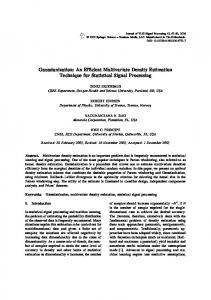


![Multidimensional Information Visualization Using ... - Semantic Scholar [PDF]](https://m.moam.info/img/260x300/multidimensional-information-visualization-using-s_6479e0c9098a9e92458b46a6.jpg)


