An Anytime Approximation for Optimizing Policies Under ... - UCI

An Anytime Approximation for Optimizing Policies Under Uncertainty Rina Dechter

Department of Computer and Information Science University of California, Irvine Irvine, California, USA 92717 dechter@@ics.uci.edu

Abstract

The paper presents a scheme for approximation for the task of maximizing the expected utility over a set of policies, that is, a set of possible ways of reacting to observations about an uncertain state of the world. The scheme which is based on the mini-bucket idea for approximating variable elimination algorithms, is parameterized, allowing a exible control between eciency and accuracy. Furthermore, since the scheme outputs a bound on its accuracy, it allows an anytime scheme that can terminate once a desired level of accuracy is achieved. The presented scheme should be viewed as a guiding framework for approximation that can be improved in a variety of ways.

1 Introduction

In uence diagram (IDs) [7] are a popular framework for decision analysis. They subsume nite horizon factored observable and partially observable, Markov decision processes (MDPs, POMDPs) used to model planning problems under uncertainty [1]. The rst part of the paper provides an overview of a bucket elimination algorithm presented in [4] for computing a sequence of policies which maximize the expected utility for an in uence diagram. The algorithm is similar to variable elimination algorithms proposed by Shachter and others [12; 13; 11; 15; 10; 14; 16; 6], and in particular, it is analogous to the join-tree clustering algorithm for evaluating in uence diagrams [6]. The new exposition using the bucket data-structure uni es the algorithm with a variety of inference algorithms in constraint satisfaction, propositional satis ability, dynamic programming and probabilistic inference. Such algorithms can be expressed succinctly, are relatively easy to implement and the uni cation highlights ideas for improved performance, for incorporating variable elimination with search, for trading space for time and for approximation, all of which are applicable within the framework of bucket-elimination [2; 3]. Indeed, in this paper we extend the principle of minibucket approximation [5] that is applicable to any vari-

able elimination algorithm, to the meu task. Speci cally, we will derive and analyze the mini-bucket approximation for the meu task in in uence diagrams and discuss its potential.

2 Background

2.1 Belief networks

Belief networks provide a formalism for reasoning about

partial beliefs under conditions of uncertainty. It is de ned by a directed acyclic graph over nodes representing random variables of interest. A directed graph is a pair, G = fV; E g, where V = fX1 ; :::; Xng is a set of elements and E = f(Xi ; Xj )jXi ; Xj 2 V; i 6= j g is the set of edges. If (Xi ; Xj ) 2 E, we say that Xi points to Xj . For each variable Xi , the set of parent nodes of Xi , denoted paXi or pai , comprises the variables pointing to Xi in G. The family of Xi , Fi , includes Xi and its parent variables. A directed graph is acyclic if it has no directed cycles. In an undirected graph, the directions of the arcs are ignored: (Xi ; Xj ) and (Xj ; Xi) are identical. The moral graph of a directed graph is the undirected graph obtained by connecting the parent nodes of each variable and eliminating direction. Let X = fX1; :::; Xng be a set of random variables over multivalued domains. A belief network is a pair (G; P) where G is a directed acyclic graph and P = fP(Xi jpai)g, denote conditional probability tables (CPTs). The belief network represents a probability distribution over X having the product form P (x1; ::::; xn) = ni=1 P(xijxpai ) where an assignment (X1 = x1; :::; Xn = xn) is abbreviated to x = (x1; :::; xn) and where xS denotes the restriction of a tuple x to the subset of variables S. An evidence set e is an instantiated subset of variables. We use upper case letter for variables and nodes in a graph and lower case letters for values in variable's domains.

2.2 In uence diagrams

An In uence diagram extends belief networks by adding also decision variables and reward functional components. Formally, an in uence diagram is de ned by ID = (X; D; P; R), where X = fX1 ; :::; Xng is a set of chance variables on multi-valued domains (the belief

network part) and D = fD1 ; ::::; Dmg is a set of decision nodes (or actions). The chance variables are further divided into observable meaning they will be observed during execution, or unobservable. The discrete domains of decision variables denote its possible set of action. An action in the decision node Di is denoted by di . Every chance node Xi is associated with a conditional probability table (CPT), Pi = fP(Xi jpai)g, pai  X [ D ,fXig. Each decision variable Di has a parent set paDi  X [ D denoting the variables, whose values will be known and may directly aect the decision. The reward functions R = fr1; :::; rjg are de ned over subsets of variables Q = fQ1; :::; Qjg, Qi  X [ D, called P scopes, and the utility function is de ned by u(x) = j rj (xQj ).1. The graph of an ID contains nodes for chance variables (circled) decision variables (boxed) and for reward components (diamond). For each chance or decision node there is an arc directed from each of its parent variables towards it, and there is an arc directed from each variable in the scope of a reward component towards its reward node. Let D1 ; :::; Dm be the decision variables in an in uence diagram. A decision rule for a decision node Di is a mapping i : paDi ! Di where for S  X [ D, S is the cross product of the individual domains of variables in S. A policy is a list of decision rules
= (1 ; ::::; m) consisting of one rule for each decision variable. To evaluate an in uence diagram is to nd an optimal policy that maximizes the expected utility (meu) and to compute the optimal expected utility. Assume that x is an assignment over both chance variables and decision variables x = (x1; :::; xn; d1; :::; dm), The meu task is to compute X  P(x ; ejx
)u(x
); (1) E =
=(max xi i pai  ;:::; ) 1

m x1 ;:::;xn

where x
denotes an assignment x = (x1 ; :::; xn; d1; :::dm) where each di is determined by i 2
as a functions of (x1; :::; xn).

DC

TC

T

R

S

D

O

OS

OP

OSP

SC

MI

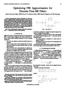
Figure 1: An in uence diagram [r(t) + r(d; op) + r(op; osp) + r(op; osp; mi)] IDs are required to satisfy several constraints. There must be a directed path that contains all the decision nodes and there must be no forgetting in the sense that a decision node and its parents be parents to all subsequent decision nodes. The rationale behind the no-forgetting constraint is that information available now should be available later if the decision-maker does not forget. In this paper, however we do not force these requirements. For a discussion of the implications of removing these restrictions see [8].

De nition 1 (elimination functions) Given a function h de ned over S , where X 2 S , P subset of variables the functions ( X h) is de ned P over U = SP, fX g as

follows. For every U = u, ( X h)(u) = x h(u; x). Given a set of functions h1 ; :::; hj de ned over P the subsets S1 ; :::; Sj, the product function (j hj ) and J hj are de ned over U = [Pj Sj . For every P U = u, (j hj )(u) = j hj (uSj ), and ( j hj )(u) = j hj (uSj ).

3 An elimination algorithm for MEU

In [4] we presented the bucket-elimination algorithm Elim-meu-id for processing in uence diagrams. For comExample 1 Figure 1 describes the in uence diagram of pleteness sake we brie y overview the algorithm (see Figthe oil wildcatter problem (adapted from [8]). The di- ure 2). agram shows that the test decision (T ) is to be made The input to the algorithm is the set of probability based on no information, and the drill (D) decision is components and utility components in the in uence dito be made based on the decision to test (T) and the agram. The operations of summation and maximization test results (R). The test-results are dependent on test that de ne the computation (EQ. (1)) requires compuand seismic-structure (S), which depends on an unob- tation along legal orderings only. We use the ordering servable variable oil underground (O). The decision re- criteria provided in [6]: assuming a given ordering for garding oil-sales-policy (OSP ) is made once the market the decision variables, unobservable variables are last information (MI) and the oil-produced (OP ) are avail- in the ordering, and chance variables between Di and able. There are four reward components: cost of test, Di+1 are those that become observable following decir(T), drill cost, r(D; OP ), sales cost, r(OP; OSP) and sion Di . Given a legal variable ordering the bucketoil sales, r(OP; OSP; MI). The meu task is to nd elimination algorithm places each probabilistic function the three decision rules T ; D and OSP : T :! T , into the bucket of its latest variable. Reward compoD : R ! D , OSP : MI;OP ! OSP such that: nents are placed according to the special procedure in X 3 (for explanation see [4]). Thus, each bucket E =  ;max P(rjt; s)P(opjd; o)P(mi)P(sjo)P(o)Figure
contains utility components i and probability compoT D ;OSP t;r;op;mi;s;o nents, i . The algorithm process the buckets from last 1 The original de nition of ID had only one reward node. to rst. The procedure in a bucket computes a new probabilistic component () and a new utility component (). We allow multiple rewards as discussed in [15]

The algorithm generates the i of a bucket by multiplying all its probability components and summing (if the variable is a chance node) over Xi . For each j 2 bucketi we compute ij as the average over Xi values normalized by the bucket's compiled . The computation is simpli ed when  = 1, namely, when there is no evidence in the bucket, nor new probabilistic functions. For a decision variable we compute a  component by maximization and simplify when no probabilistic components appear in the decision bucket. We showed in[4] that processing a decision variable, does not, in general, allow exploiting a decomposition in the reward components. The eect of an observation on processing either a decision bucket or a chance bucket is the assignment of the value to each component and then placing each into a lower bucket. Therefore, as usual, observed variables simplify computation by avoiding creating new dependencies among variables. We will next demonstrate the algorithm on the wildcatter example.

Example 2 Consider the in uence diagram of Figure 1

where u = r(t) + r(d; op) + r(op; mi; osp) the ordering of processing is o = T; R; D; OP; MI; OSP; S; O. The chance variables O and S are unobservable and therefore placed last in the ordering. The bucket`s partitioning and the schematic computation of this decision problem is given in Figure 4 and is explained next. Initially, bucket(O) contains P (opjd; o); P (sjo); P(o). Since this is a chance bucket having no reward components we generate

O

X (s; op; d) = P (opjd; o)P(sjo)P (o) o

placed in bucket(S). The bucket of S is processed next as a chance bucket. We compute

S (r; op; d; t) =

X P (rjt; s) s

O (s; op; d)

placed in bucket(OP ). The bucket of the decision variable OSP is processed next. It contains all the reward components r(op; mi; osp), r(op; osp), r(t) and r(d; op). Since the decision bucket contains no probabilistic component, r(t) is moved to the bucket of D and r(d; op) is moved to the bucket of OP . We then create a utility component

OSP (op; mi) = max [r(op; mi; osp) + r(op; osp)] osp

Which is the decision rule for OSP , and place it in bucket(MI). The bucket of MI is processed next as a chance bucket, generating a constant  = 1 and

MI (op) =

X P(mi)

OSP (op; mi);

mi

placed in the bucket of OP . Processing the bucket of OP yields: X

OP (r; t; d) =

op

S (r; t; op; d)

Algorithm elim-meu-id Input: In uence diagram (X; D; P; R), a legal ordering of the variables, o; observations e. Output: Decision rules 1 ; :::; k that maximizes the expected utility. 1.Initialize: Partition components into buckets

where bucketi contains all probabilistic components whose highest variable is Xi . Reward components are partitioned using procedure partitionrewards. In each bucket, 1 ; :::; j, denote probabilistic components and 1 ; :::; l utility components. Let S1 ; :::; Sj be the scopes of probability components, and Q1 ; :::; Ql be the scopes of the utility components. 2. Backward: For p n downto 1, do Process bucketp: for all functions 1; :::; j ; 1; :::; l in bucketp , do  If (observed variable) bucketp contains Xp = xp , assign Xp = xp to each i ; i , and put each resulting function in appropriate bucket.  else, { If XpPis a Qchance variable compute p = Xp i i and for each P i 2 bucketp compute, 1 i p = p Xp i ji=1 i ;

{ If Xp is a decision variable, then If bucket has only 's , move each free

from Xp , to its appropriate lower bucket, and for P the rest compute p = maxXp j j else, (the general Q case), P compute p = maxXp ji=1 i lj =1 j

{ Add p to the bucket of the largest-index

variable in their scopes. Place p in the closest chance bucket of a variable in its scope or in the closest decision bucket. 3. Return : decision rules computed in decision buckets. Figure 2: Algorithm elim-meu-id

Procedure partition-rewards(P1; :::; Pn; r1; :::rj, o) For i = n to 1

If Xi is a chance variable, put all rewards mentioning Xi in bucketi. else (decision variable) put all remaining rewards in current bucketi end. Return ordered buckets Figure 3: partition into buckets

bucket(O) : P(ojop; D)P (sjo); P(o) bucke(S) : P (rjs; t) jj O (s; op; d) bucket(OSP ): r(t); r(op; osp); r(op; mi; osp); r(d; op) bucket(MI): P(mi) jj OSP (op; mi) bucket(OP ): jj S (r; t; op; d); r(op; d); MI(op) bucket(D): jj OP (r; t; d); OP (d; r; t)r(t) bucket(R): jj D (r; t) bucket(T ): jj R (t) Figure 4: A schematic execution of elim-meu and

X  (r; t; op; d)[r(op; d) +  (op)] OP (r; t; d) =  1 S MI OP op both placed in the bucket of decision variable D. Here we

observe the case of a decision bucket that contains both probabilistic and utility component. The bucket has two reward components (one original r(t) and one generated recently.) It computes a  component:

D (r; t) = max  (r; t; d)[r(t) + OP (r; t; d)] D OP which provides the decision rule for D and is placed in the bucket of R. The bucket of RPhas only a probability component yielding: R (t) = r D (r; t) placed in bucket(T ), and T = maxt R (t) is derived and provides the decision rule for T . Also, maxt R (t) is the optimal expected utility. The sequence of solution policies is given by the argmax functions that can be created in decision buckets. Once decision T is made, the value of R will be observed, and then decision D can be made based on T and the observed R.

In summary,

Theorem 1 [4] Algorithm elim-meu-id computes the

meu of an in uence diagram as well as a sequence of optimizing decision rules. 2

3.1 Complexity

As is usually the case with bucket elimination algorithms, their performance can be bounded as a function of the induced width of some graph that re ect the algorithm's execution. An ordered graph is a pair (G; d) where G is an undirected graph and d = X1 ; :::; Xn is an ordering of the nodes. The width of a node in an ordered graph is the number of the node's neighbors that precede it in the ordering. The width of an ordering d, denoted w(d), is the maximum width over all nodes. The induced width of an ordered graph, w (d), is the width of the induced ordered graph obtained as follows: nodes are processed from last to rst; when node X is processed, all its preceding neighbors are connected. The induced width of a graph, w, is the minimal induced width over all its orderings. The relevant graph for elim-meu-id, is the augmented graph obtained from the ID graph as follows. All the

parents of chance variables are connected (moralizing the graph), all the parents of reward components are connected, and all the arrows are dropped. Value nodes and their incident arcs are deleted. The reader can check that the width of the augmented graph for the oil example along the order of processing is 3 while the inducedwidth is 4. The complexity of elim-meu-idis O(n
exp(w)), where w is the induced-width of the augmented ordered graph. (see [4] for more details.)

4 Mini-bucket for MEU

Since the complexity of elim-meu-id is exponential in the induced-width of some graph and since the inducedwidth is at least as large as that of the underlying moral graph of the probabilistic subnetwork, frequently space complexity will not allow executing the full bucket elimination algorithm and we need an approximation scheme. The idea of the mini-bucket approach is to localize the computation done in each bucket [5]. Since elimmeu-id process chance variables and decision variables dierently we will derive the mini-bucket simpli cation for each of the two cases. We will demonstrate the idea using the car example.

4.1 The car buyer example

Consider a car buyer that needs to buy one of two used cars. The buyer of the car can carry out various tests with various costs, and then, depending on the test results, decide which car to buy. Figure 5 gives the in uence diagram representing the car buyer example adapted from [9]. T denotes the choice of test to be performed, T 2 ft0 ; t1; t2g (t0 means no test, t1 means test car 1, and t2 means test car 2). D stands for the decision of which car to buy, D 2 fbuy 1; buy2g. Ci represents the quality of car i, i 2 f1; 2g and Ci 2 fq1; q2g (denoting good and bad qualities. ti represents the outcome of the test on car i, ti 2 fpass; fail; nullg. The null option corresponds to the case when a test on car i was not performed. The cost of testing is given as a function of T, by r(T ), the reward in buying car 1 is de ned by r(C1; D = buy 1) and the reward for buying car 2 is r(C2; D = buy 2). The rewards r(C2 ; D = buy 1) = 0, and r(C1 ; D = buy 2) = 0. The total reward or utility is given by r(T) + r(C1 ; D) + r(C2; D). The task is to determine T and D that maximize the expected utility. Namely, X P (t jC ; T )P (C )P (t jC ; T )
(2) E = max 2 2 2 1 1 T;D t2;t1 ;C2 ;C1

P(C1)[r(T ) + r(C2; D) + r(C1 ; D)]: The bucket-elimination algorithm partitions the probabilistic and reward components into ordered buckets as described in the algorithm. Using the ordering o = T; t2; t2; D; C2; C1, the initial partitioning for the car example is given in Figure 6. Figure 7 shows the recorded functions in the buckets after processing in reverse order of o.

r(T)

and X C (t1 ; T; D) =  (t1 ; T )
P (t1jC1; T )P (C1)r(C1; D) C 1 C (6) Instead, we will now derive an approximation for these expressions. X EC = P (t1 jC1; T)P(C1)[r(T )+r(C1; D)+r(C2 ; D)] = 1

T C1

C2

1

1

X P(t jC ; T )P(C )[r(T) + r(C ; D)]+ 1 1 1 2 C X P(t jC ; T)P (C )r(C ; D):

C1

t2

t1

1

=

1

r(C1 ,D )

r(C2,D)

Figure 5: In uence diagram for car buyer example bucket(C1): P(C1); P(t1jC1; T); r(C1; D) bucket(C2): P(C2); P(t2jC2; T); r(C2; D) bucket(D): bucket(t1 ): bucket(t2 ): bucket(T ): r(T) Figure 6: Initial partitioning into buckets The optimizing policies for T is the simple decision function computed in bucket(T), the argmax of EQ. (3): E = max  (T )t (T)[r(T) + t (T)]: (3) T t 1

2

2

and D (t1 ; t2; T) that is recorded in bucket(t1 ) or its associated maximizing decision D. We will next apply the mini-bucket idea. From EQ. (2) we get: X X max X P (t jC ; T)P (C )
(4) E = max 2 2 2 T D t2 t1

C2

X P (t jC ; T )P (C )[r(T ) + r(C ; D) + r(C ; D)] C1

1 1

1

1

2

Focusing on the expression involving C1 (that corresponds to processing bucket(C1 )) leads to computing the  and  as in EQ. (5) and (6): X C (t1 ; T) = P (t1jC1; T)P(C1) (5) 1

C1

bucket(C1): P(C1); P(t1jC1; T); r(C1; D) bucket(C2): P(C2); P (t2jC2; T); r(C2; D) bucket(D): jj C (t1 ; T; D); C (t2 ; T; D) bucket(t1 ): jj C (t1 ; T ); D (t1 ; t2; T) bucket(t2 ): jj C (t2 ; T ); t (t2 ; T ) bucket(T ): r(T)jjt (T); t (T ); t (T). Figure 7: Schematic bucket evaluation of car example 1

2

1 2

1

1

1 1

C1

D

2

2

1

1

By applying the summation over C1 in two stages, migrating summation inside X the product we get X EC  [r(T ) + r(C2; D)][ P (t1jC1; T)][ P (C1)]+ 1

C C X X [ P (t1jC1; T)][ P(C1)r(C1; D)] = C C X X [ P (t1jC1; T)][ P (C1)]
[r(T) + r(C2 ; D)+ C C X 1 P [ P(C )r(C ; D)]] 1

1

1

1

1

1

1

C1 P(C1) C1

1

The last expression corresponds to partitioning the bucket of C1 into two mini-buckets; one containing P (t1jC1; T) and the other containing P (C1) and r(C1; D). Each mini-bucket is processed as a chance bucket in elim-meu-id ( see in Figure 8, the initial partitioning into mini-buckets). We assign indices to minibuckets in a buckets in the order from left to right. Processing mini-bucket of C1 yields 1C (t1 ; T ) = PC P(tthe1jC1 rst ; T ) (superscripts denote the mini-bucket creating the function), and processing the second mini2C = P P (C1) = 1, bucket yields both a  function  C P and a  function C2 (D) = C P (C1)r(C1 ; D), both placed in a corresponding bucket below. Processing the bucket of C2 is similar. Likewise, we can derive the mini-bucket processing of decision variable. In our example, by the time bucket(D) is processed it contains two  functions created earlier. Since the bucket has no probabilistic component, it is processed as a regular full decision bucket and since it has functions on over D only. Namely we compute D = maxD (C2 (D)+C2 (D)). The nal status of the buckets after processing is given in Figure 8. We see that the mini-bucket partitioning yields a decision D, that is independent of the testing of the cars: D = argmaxD (C (D)+C (D)) (superscripts are omitted whenever no confusion may arise). Indeed, since the functions i (ti ) for i = 1; 2 evaluates to the constant (1), the decision T = t0 is selected when evaluating bucket T (we assume negative reward functions). So the approximation yields a very simple decision rule. No testing (the decision for T) and then the appropriate maximization of expected cost for deciding which car to buy. We next present the general derivation. 1

1

1

1

1

1

2

1

2

1

bucket(C1): fP(t1jC1; T)g; fP (C1); r(C1; D)g bucket(C2): fP(t2 2jC2; T)g2; fP (C2); r(C2; D)g bucket(D): jj C (D); C (D) bucket(t1 ): jj 1C (t1 ; T ) bucket(t2 ): jj 1C (t2 ; T ) bucket(T ): r(T) jj t (T); t (T); D T = armaxT t (T)t (T)[r(T ) + D ] Figure 8: Initial partitioning into buckets 1

Qlj k , we can upper-bound Ep by Ep 

2

1 2

1

1

2

2

4.2 General derivation for chance buckets

As speci ed by the full bucket-elimination algorithm, if Xp is a chance bucket, the full bucket elimination algorithm, computes in bucketp (that contains the compoj; 1; :::; k) two types of functions. p = Pnents:Qj1; :::;i and, for each i 2 bucketp, Xp i=1 P Q 1 i p = p Xp i ( ji=1 i ). Since the functions p and pi may have high dimensionality we will try to approximate them with functions of lower dimension. To achieve that, two parameters, i and m are used. Given this two parameters, we partition the probabilistic components and the utility components 1 ; :::; j; 1; :::; k in bucket Xp into an (i; m)-partitioning, not allowing more than i variables or more than m components in a mini-bucket. Denoting the mini-buckets Q0 = fQ1; :::; Qrg. For each Ql 2 Q0, containing l ; :::; ltl ; l ; :::; lfl we compute 1

1

XY ; l = tl

Xp i=1

X Ytl lj = 1l lj li Xp i=1

k2lp

Since i for i 2 tp does not depend on Xp we get: Ep

X X Yj  + X X  Yj  = 
k2tp

k

Xp i=1

i

k2lp Xp

X X ( Y k

k2lp Xp

k

Qj 2Q0 Xp ji 2Qj

2Qlj(k)

ji

Y X Y )

)
(

Ql 2Q0;l6=lj(k) Xp 2Ql

P Q

j Namely, we bound Xp i=1 i Q P Q by Ql 2Q0 Xp 2Ql  when exchanging summation with multiplication. Lets denote: Y XY gp = Ql 2Q0 Xp 2Ql

We get:

X  + X Q P1 Q k k tp k lp Ql Q Xp  Ql 
X Y ]
( Y X Y )]
[ 

Ep  gp
[ Xp

k

2

2 0

2

2

Ql 2Q0;j 6=jl Xp 2Ql

2Qlj(k)

After canceling out multiplicands in the dominator and denominator in the second summand we get: X X P Q1 X  Y ] = gp
[ k +
k k2tp k2lp Xp 2Qlj k  Xp 2Ql j(k)

( )

4.3 General derivation for decision bucket

Each of these components is moved to a lower bucket using the usual rule. We next show that for any partitioning, this approximation yields an upper bound on the exact computation in a chance bucket. Let's denote by tp the indices of variables in the scopes of the  functions which are currently placed in lower buckets, namely i 2 tp if i 2 bucketk for k < p, and by lp the set of indices of i functions in bucketp (namely, those are de ned over Xp ). The function computed in the bucket of Xp by full bucket elimination is equivalent to: X Yj  ( X  + X  ) Ep = i k k k2tp

+

k2tp

This concludes the justi cation for processing chance mini-buckets. It shows that for each mini-bucket of a chance variable we simply apply the same procedure that is associated with the processing of full chance buckets.

li

and, for each lj 2 Ql we compute

Xp i=1

X
Y X Y

( )

k

i=1

i

Given the partitioning into mini-buckets Q0 = Q1; :::; Qr, and assuming that k appears in a speci c mini-bucket

A decision bucket may contain both probabilistic and utility components. In that case the full bucket elimination algorithm computes a  function Y ( X  ) p = max i k X p

i

k2tp [lp

Lets choose a partitioning where all utility components are placed in one mini-bucket. Let Q0 = fQ1 ; :::; Qrg be the partitioning and let Q1 be the the mini-bucket containing all the utility components. Y ( X  ) Y Y  ] p = max [ k i X p 2Q 1

k2tp [lp

j =2;:::;r i 2Qj

In that case p can be approximated, when migrating the maximization into each mini-bucket, by Y  X  ]
Y max Y  (7) p  max [ i k i Xp Xp i2Q1

k

j =2;:::;r

i 2Qj

This means that we compute a  component in each pure mini-bucket by Y (8) lp = max i X p  2Q i l

and in the mixed bucket by Y  X ] Qp 1 = max [ i k X p  2Q i 1

(9)

k

Algorithm approx-meu-id(i,m) Input: In uence diagram (X; D; P; R), a legal ordering , o; observations e. Output: Decision rules 1 ; :::; k approximating the max expected utility. 1.Initialize: Partition into buckets as in elim-

If the mixed mini-bucket has too many variables, it is further partitioned as guided by the following expresCall probability matrices 1; :::; j sions. Following some algebraic manipulation we get meu-id. and utility matrices 1 ; :::; l. Let S1 ; :::; Sj be from EQ. (7): the scopes of the probability components and Q P Y max Y  X [ + maxXp i2QQ i k2lp kQ] 1; :::; Ql be the scopes of the reward components. p  i k maxXp i 2Q i 2. Backward: For p n downto 1, do j =1;:::;r Xp i 2Qj k2tp  If (observed variable, or a predetermined decision policy) bucketp contains Xp = xp , then This suggests that, as before, the pure  buckets are assign Xp = xp to each i ; i , and place result computed by EQ. (8). In the mixed mini-bucket Q1, we in lower bucket. rst move all  elements not de ned over Xp to lower buckets and then compute a  function  else, If Xp is a chance variable then generate an (i; m)-partitioning of bucketp , Q0 = Qp = max   Xp 2Q Q1; ::::; Qt. For each mini-bucket Ql , containing and a  function by: l ; :::; lj ; l ; :::; ll compute: Q 2Q i Pk2l k max X p i p { l = PXp Qti=1 li Q (10) p1 = maxXp i 2Q i { For each P k 2 QlQcompute P lk = 1l Xp k 2Ql  If k2lp k is still too high dimensional and cannot t into one mini-bucket, we can further partition Q1 into mixed mini-buckets fQ1 ; :::Q1j ; :::; Q1tg and compute else, If Xi is a decision variable then Place separate functions for each subset Q1j  Q1. By exall utility components in Q1 together with changing summation and multiplication we get:  components whose scopes are included in Pj maxXp [P 2Q k Q 2Q i] that bucket. Generate an (i,m) partitioning kQ j i 1 to the rest of the s, yielding mini-buckets: (11) p  maxXp i 2Q i Q1; :::; Qt. Call probability matrices in Ql l ; :::; lj Therefore, it will allow computing for each Q1j  Q1, { For every pure mini-bucket Ql compute the function p1j by: l = P Qt l  Xp i=1 i P 2Q k ] Q 2Q i max [ X p { If the mixed mini-bucket Q1 ts into one k i j Q p1j = : (12) mini-bucket of an (i,m)-partitioning commaxXp i 2Q i pute a  component using the full bucket decision rule: Algorithm approx-meu-id(i,m) is described in Figure 9. P Qp 1 = maxXp 2Q  2Q  Theorem 2 Algorithm Approx-meu-id(i,m) computes else, move all  functions not de ned on an upper bound on the maximum expected utility of a set Xp to lower buckets, then apply an arof policies. Its complexity is time and space exponential bitrary (i,m)-partitioning for the rest of in the bounding parameters i and m. 2 the functions called Q1 ; :::; Q1n . Example 3 Consider again the wildcatter example. For any mixed Q1j  Q1 , compute: The initial partitioning into buckets is as in the full Q 2Q i P 2Q k bucket elimination case. Here we show the nal buckmax X p i k j 1 Q pj = ets assuming i=3. max  Xp i 2Q i The processing of each bucket is explained as follows. (13) Bucket(O) has two mini-buckets. PProcessing the rst 1 yields a  component: O (op; d) = O P(ojop; d) which Add  and  to the bucket of the largest-index is placed in bucket(OP ). Processing thePsecond miniin their argument list. bucket yields a  component: 2O (S) = O P(sjo)p(o) 3. Forward: Return an upper bound on the placed in bucket S . Processing bucket(S) is done as a full maximum expected utility computed in the rst bucket since its number of variables is bounded by 3. We P bucket. Execute the policies recorded in the buckget: S (r; t) = S P (rjs; t)2O (s), placed in bucket(r). ets of the decision parents using the ordering From now on, all buckets will be processed as full buckX1 ; ::::Xn. ets. The bucket of the decision variable OSP is processed 1

1

1

1

1

1

1

1

1

1

1

1

1

1

1

1

1

1

1

1

1

1

next. Since the decision bucket contains no probabilistic

Figure 9: Algorithm approx-elim-meu-id

bucket(O) : P(ojop; D)P (sjo); P(o) bucke(S) : P (rjs; t) jj O (s; op; d) bucket(OSP ): r(t); r(op; osp); r(op; mi; osp); r(d; op) bucket(MI): P(mi) jj OSP (op; mi) bucket(OP ): jj (S (r; t; op; d); r(op; d); MI(op) bucket(D): jj OP (r; t; d); OP (d; r; t)r(t) bucket(R): jj D (r; t) bucket(T ): jj R (t) The mini-bucket processing results in: bucket(O) : fP(ojop; d)gf2P (sjo); P(o)g bucke(S) : P(rjs; t) jj O (s) bucket(OSP ): r(t); r(op; osp); r(op; mi; osp); r(d; op) bucket(MI): P(mi) jj OSP (op; mi)) bucket(OP ): jj 1O (op; D), r(op; d), MI (op) bucket(D): jj OP (d); OP (d); r(t) bucket(R): jj S (r; t) bucket(T ): jj Mi ; D (t); R (t) Figure 10: Comparing the complete algorithm and its approximation on the oil example component, r(t) is moved to the bucket of D and r(d; op) is moved to the bucket of OP . We then create a utility component

OSP (op; mi) = max [r(op; mi; osp) + r(op; osp)] osp and place it in bucket(MI), and so on. Processing the bucket T is by: T = maxt [R (t) + Mi + D (t)] providing the decision rule for T . Also, T is an upper bound on the optimal expected utility (see Figure 10). The new recorded functions are shown to the right of the bar. The subscript of each function indicate the bucket originating the function. We see that the approximation generates only functions on two variables while the exact algorithm created functions on four variables (S (r; t; op; d)). We observe that the decision policy for OSP is not changed by this mini-bucket execution, however decision D is recorded as a function of T only while for the full algorithm it is a function of both T and R.

5 Discussion and Conclusion

The paper presented a bucket-elimination algorithm for maximizing the expected utility over a set of policies and analyze its complexity using graph parameters such as induced width. We present a general approximation scheme based on the mini-bucket idea for approximating the bucket-elimination algorithm for nding optimal policies. The scheme allow a exible control of accuracy and eciency using a parameter i that bounds the size of the functions that can be recorded by the algorithm. The approximation generates an upper and lower bounds thus allowing an aposteriori knowledge of its quality. The approach is applicable also to the more planningspeci c models of nite horizon MDPs and POMDPs to be further studied.

References

[1] C. Boutilier, T. Dean, and S. Hanks. Decisiontheoretic planning: Structural assumptions and computational leverag. Arti cial Intelligence Researc (JAIR), 11:1{94, 1999. [2] R. Dechter. Bucket elimination: A unifying framework for probabilistic inference algorithms. In Uncertainty in Arti cial Intelligence (UAI'96), pages 211{219, 1996. [3] R. Dechter. Bucket elimination: A unifying framework for reasoning. Arti cial Intelligence, pages 41{ 85, 1999. [4] R. Dechter. A new perspective on algorithms for optimizing policies under uncertainty. In AI-Planning, 2000 (submitted), 2000. [5] R. Dechter and I. Rish. A scheme for approximating probabilistic inference. In Proceedings of Uncertainty in Arti cial Intelligence (UAI'97), pages 132{141, 1997. [6] F.V. Jensen F. Jensen and S.L. Dittmer. From in uence diagrams to junction trees. In Tenth Conference on Uncertainty in Arti cial Intelligence, pages 367{363, 1994. [7] R. A. Howard and J. E. Matheson. In uence diagrams. 1984. [8] R. Qi N. L. Zhang and D. Poole. A computational theory of decision networks. International Journal of Approximate Reasoning, pages 83{158, 1994. [9] J. Pearl. Probabilistic Reasoning in Intelligent Systems. Morgan Kaufmann, 1988. [10] R. Shachter and M. Peot. Decision making using probabilistic inference methods. In Proceedings of Uncertainty in Arti cial Intelligence (UAI92), pages 276{283, 1992. [11] R. D. Shachter. An ordered examination of in uence diagrams. Networks, 20:535{563, 1990. [12] R.D. Shachter. Evaluating in uence diagrams. Operations Research, 34, 1986. [13] R.D. Shachter. Probabilistic inference and in uence diagrams. Operations Research, 36, 1988. [14] P.P. Shenoy. Valuation-based systems for bayesian decision analysis. Operations Research, 40:463{484, 1992. [15] J.A. Tatman and R.D. Shachter. Dynamic programming and in uence diagrams. IEEE Transactions on Systems, Man, and Cybernetics, pages 365{379, 1990. [16] N. L. Zhang. Probabilistic inference in in uence diagrams. Computational Intelligence, pages 475{ 497, 1998.