Abstract-This paper describes a new microprocessor controlled ac bridge method using an LMS adaptive algorithm. The main advan- tages of the method ...
894
IEEE TRANSACTIONS ON INSTRUMENTATION AND MEASUREMENT, VOL. IM-36, NO.4, DECEMBER 1987
An Application of an LMS Adaptive Algorithm for a Digital AC Bridge MITA DUTTA, ANJAN RAKSHIT, MEMBER, IEEE, S. N. BHATTACHARYYA, AND J. K. CHOUDHURY
Abstract-This paper describes a new microprocessor controlled ac bridge method using an LMS adaptive algorithm. The main advantages of the method include: (i) the algorithm is simple to implement because no complex computations are actually involved, and (ii) slowly time varying impedances ~ay also be measured or monitored. A realtime implementation of the bridge has been made and test results obtained have been incorporated in the paper.
I. INTRODUCTION NTIL RECENTLY, techniques for performing pre. . cision impedance measurements generally made use of ac bridges which are balanced manually and are slow in operation. The digital ac bridge described in this paper features balancing by means of a least mean square (LMS) adaptive algorithm [1]-[3], as applied to complex quantities [4]. The process is iterative and is preformed under computer control. Such software operating ac bridges enjoy the following advantages in comparison to conventional ac bridges: high accuracy, reproducibility, reliability and flexibility [5]-[7]. However, conventional software operated ac bridges have a limitation in their ability to track time varying parameters. The present bridge method obviates this limitation and provides a simple and effective method of tracking time varying impedances.
U
II. SOFTWARE OPERATED DIGITAL AC BRIDGES Fig. 1 shows the principle of a software operated digital ac bridge. The bridge is formed by two symmetrical sinewave generators (Vx' Vr) and by the impedances (Zx, Z,) to be compared. In the balanced bridge, the unknown impedance is measured in terms of the ratio of the two voltages and the absolute value of the reference impedance. In an idealized case, without considering stray impedances, the balance condition is
(1) where Vx and Vr are the rms values of variable and reference voltage sources, respectively. Z, is the unknown impedance, and Z, is the reference impedance. The error voltage E (Fig. 1) is given by
E = (VxZr - VrZx)/(Zx + Zr).
(2)
Manuscript received April 28, 1987. The authors are with the Electrical Engineering Department, Jadavpur University, Calcutta 700 032, India. IEEE Log Number 8716858.
E
BridVI Boionci alvorithm Fig. 1.
AC bridges are conventionally balanced by successive adjustments of one or several parameters, each adjustment tending to decrease the out-of-balance voltage. The number of steps required to balance the bridge indicates the convergence rate which depends on the bridge components and their configuration. III. THE LMS ALGORITHM FOR BRIDGE BALANCE Fig. 2 illustrates the basic technique on which the present scheme is based [8]. The bridge is balanced by controlling the complex voltage Vx ' in phase and amplitude, according to a simplified version of the complex LMS algorithm [4]. The simplification occurs in the sense that no complex computation is actually involved. Essentially, an LMS adaptive algorithm compares a desired signal with a signal synthesized on the basis of the requirement that the difference between the desired signal and the synthetic signal, viz. the error, leads to a minimum in the mean square sense. The synthetic signal is derived from one or more reference source channels, a weight being attached to each channel. These weights are adaptively altered by the algorithm in order to achieve the LMS error condition. With reference to Fig. 2, the desired signal i~ the voltage drop across the unknown impedance Z, at bridge balance and is given by (u.Z, / Zr), where u, is the instantaneous reference voltage. The synthetic in-phase and quadrature signal channels Vxi and v xq, respectively, are derived from the reference voltage source with the respective weights Wxi and Wxq attached to the channels. The LMS algorithm tends to minimize the difference between the desired voltage drop (vrZx)/Zr and the synthetic voltage Vx (= Vxi + v xq) in the LMS sense. In other words the algorithm minimizes the bridge out-of-balance voltage "e" in the LMS sense. Vr , the reference voltage source, is assumed to be an n-
0018-9456/1200-0894$01.00 © 1987 IEEE
DUTTA et al.: LMS ADAPTIVE ALGORITHM
895
The eigenvalues can be expressed as [9] WXJk
A), A2
==
(A
2/2)[I
± cos
(woT)]
(9)
where A is the amplitude of the sinusoid. The largest eigenvalue Amax is given by
Wr,Qk
forn~4.
(10)
Fig. 3 shows the variation of Amax with n. From the curve one can select u, where
°