To appear in IEEE transactions on Neural Networks, Volume 5, Number. 3, 1994 .... At the other extreme the phone class probability estimators are trained in-.
An Application of Recurrent Nets to Phone Probability Estimation Tony Robinson To appear in IEEE transactions on Neural Networks, Volume 5, Number 3, 1994
Abstract This paper presents an application of recurrent networks for phone probability estimation in large vocabulary speech recognition. The need for e�cient exploitation of context information is discussed; a role for which the recurrent net appears suitable. An overview of early developments of recurrent nets for phone recognition is given along with the more recent improvements which include their integration with Markov models. Recognition results are presented for the DARPA TIMIT and Resource Management tasks, and it is concluded that recurrent nets are competitive with traditional means for performing phone probability estimation.
1 Introduction The aim of this paper is to describe the application of a recurrent net to phone recognition. There are several forms of recurrent net (e.g. [1, 2, 3]), however this paper is interested in the kind that map one sequence on to another. This form of recurrent net is potentially very powerful as it is capable of emulating any nite state machine [4]. Speci cally, the aim of the network is to perform the mapping from a sequence of frames of parameterised speech to a sequence of phone labels associated with those frames. There are noticeable correlations between a speech frame and the associated label, but there are many contextual e�ects which make the task a challenging one. This paper traces the development of one use of recurrent nets to phone recognition. It starts with an overview of the problem and a survey of the currently used techniques that are applied. These techniques are considered from the point of view of scaling to incorporate more contextual information and a recurrent net is proposed as a possible solution. An overview of recurrent net architectures is given, and one based on backpropagation through time is supported. Many details are necessary to provide a state of the art implementation of recurrent nets for phone probability estimation and these are described in the next section along with a method for combining these probabilities to perform phone and word recognition. Finally results are presented for the TIMIT phone recognition task and the Resource Management word recognition task and comparisons are made with other systems. 1
2 Why use recurrent nets for speech recognition? In general, researchers are agreed that in order to cope with a large vocabulary (say greater than few hundred words) it is necessary to use sub-word models and a pronunciation model for each item in the vocabulary in order to represent every word properly. A popular choice for the sub-word units is the phone, although diphone, triphone and syllable based approaches are being pursued. The phoneme is a semantic category, it being the smallest unit that is used to distinguish meaning (e.g. [5]). A phone is the acoustic category corresponding to the phoneme. The speci c phone that is used in any instance is dependent on contextual variables such as speaking rate. By specifying the pronunciation of a word in terms of a string of phones the task is reduced to estimating the probabilities of phone strings and then searching all possible phone strings for the most probable legal word string. The most popular tool for this task is the Hidden Markov Model (HMM) (e.g. [6, 7]). Individual models are created for each phone and these are concatenated to form word models. Each HMM phone model can be matched to any segment of speech and the likelihood of the model generating the observed acoustic evidence can be computed. However, there are several known problems with using HMMs as they assume that a frame of speech is generated purely as a result of occupation of a particular HMM state within a particular phone. In practice, there are many contextual variables that a�ect the speech waveform and which are not a function of the current state of the phone being uttered.
2.1 Context in speech recognition
Context is very important in speech recognition at all levels. On a short time scale such as the average length of a phone, limitations on the rate of change of the vocal tract cause a blurring of acoustic features which is known as coarticulation. For longer time scales there are many slowly varying contextual variables (e.g. the degree and spectral characteristics of background noise and channel distortion) and speaker dependent characteristics (e.g. vocal tract length, speaking rate and dialect). To achieve speech recognition at the highest possible levels of performance means making e�cient use of all of the contextual information. Current HMM technology approaches the problem from two directions: top down, by considering phonetic context; and bottom up, by considering acoustic context. The short-term contextual in uence of coarticulation is handled by creating a model for all su�ciently distinct phonetic contexts. This entails a trade o� between creating enough models for adequate coverage and maintaining enough training examples per context so that the parameters for each model may be robustly estimated. Clustering and smoothing techniques can enable a reasonable compromise to be made at the expense of model accuracy and storage requirements (e.g. [8, 9]). However, the problem remains of the number of models increasing exponentially with increasing number of contextual variables which limits the applicability of this technique. Acoustic context is handled by increasing the dimensionality of the observation vector to include some parameterisation of the neighbouring acoustic vectors. This changes the problem to one of obtaining robust probability estimation from high dimensional spaces. 2
2.2 Probability estimation in speech recognition
Increasing the dimensionality of the acoustic vector increases the amount of contextual information available. The simplest way to do this is to replace the single frame of parameterised speech by a vector containing several adjacent frames along with the original central frame. However, this dimensionality expansion quickly results in di�culty in obtaining good models of the data. For example, Gaussian distributions of acoustic parameters are often assumed for each class, but for an n dimensional acoustic vector, O(n ) parameters in the covariance matrix must be estimated. This can be reduced by assuming that subsets of the acoustic vectors are independent (block diagonal covariance matrix), or that all acoustic parameters are independent (diagonal covariance matrix), but this clearly limits the modelling power available (e.g [10]). Careful choice of the method used to increase the information content of the acoustic vector is clearly important. Empirically it has been shown that rst (and second) order di�erences taken over a window length of a few frames are a reasonable choice for the parameterisation of acoustic context and yield substantial improvements in speech recognition accuracy [11]. As a result this parameterisation has been widely adopted by the speech recognition community. Di�erence coe�cients are a simple linear function of the acoustic vectors lying within a rectangular window. Automatic optimisation of the linear function may be achieved using linear discriminant analysis and this has also been shown to yield increased recognition performance [12]. However, long term contextual information such as the speaker dependence of the acoustic realisation of phonemes will not be adequately modelled by a linear transformation to a small subspace. Methods are needed that can capture high order correlations over long time periods. Multi-layer perceptrons (MLPs) are a suitable candidate as it has been shown by a number of authors that when used for classi cation these networks approximate the posterior probability of class occupancy [13, 14, 15, 16, 17]. For a full discussion of this result to speech recognition see [18, 19]. 2
2.3 Hybrid connectionist / Markov model systems
The use of MLPs allows a large window of parameterised speech to be used directly for the estimation of phone class probabilities [20]. Indeed, it can be seen that any linear transformation may be built into the rst layer of a MLP by modifying the weights before the non-linearity. The use of multiple layers allows the independence restrictions to be relaxed, so enabling high order correlations to be exploited. Experimenters with connectionist word recognition report that connectionist probability estimators yield better results than the equivalent HMM based on mixtures of Gaussian likelihoods [21]. There are two extremes in approaches to building hybrid connectionist/HMM systems. At one end, a standard HMM can be considered as a connectionist model with as many layers as there are frames of speech allocated to the model. Performing gradient ascent in the log likelihood of the model gives standard Maximum Likelihood trained models (e.g. [22]). At the other extreme the phone class probability estimators are trained independently of the HMM transition probabilities. This is similar to Viterbi training of HMMs in that only the most probable state sequence is used to train the emission probabilities from a state and has the advantage that discriminative training can be used 3
(e.g. [20]). There are several intermediate positions in which gradient descent techniques can be used for discriminative training of HMMs (e.g. [23, 24, 25]) and posterior state occupancy probabilities can be used as targets for connectionist training. There are also a variety of architectures worth considering for use as connectionist probability estimators. The simplest employs a standard three layer MLP structure. Whilst this has been shown to give good results [20], at best the number of parameters to estimate varies linearly with the temporal extent of acoustic information considered. Weight sharing allows encoding of prior knowledge and gives better scaling properties at the expense of imposing restrictions on the diversity of the computations performed [26]. Along with the non-connectionist probability estimation methods, these techniques are restricted to a nite length window on the acoustic data.
2.4 Recurrent nets for phone probability estimation
The incorporation of feedback into a MLP gives a method of e�ciently incorporating long term context in much the same way as an in nite impulse response lter can be more e�cient than a nite impulse response lter in terms of storage and computational requirements. Duplication of resources is avoided by processing one frame of speech at a time in the context of an internal state as opposed to applying nearly the same operation to each frame in a larger window. Feedback also gives a longer context window, so it is possible that uncertain evidence can be accumulated over many time frames in order to build up an accurate representation of the long term contextual variables. The rest of this paper will describe such a recurrent net used to estimate phone class probabilities for incorporation with a Markov model word recognition system. Results are presented at both the phone and word levels, along with a discussion of the work that still needs to be done.
3 Basic theory The form of the recurrent net used here was rst described by the author in [27]. This paper took the basic equations for a linear dynamical system and replaced the linear matrix operators with non-linear feedforward networks. After merging computations, the resulting structure is illustrated in gure 1. The current input, u(t), is presented to the network along with the current state, x(t). These two vectors are passed through a standard feed-forward network to give the output vector, y(t) and the next state vector, x(t + 1). De ning the combined input vector as z(t) and the weight matrices to the outputs and the next state as W and V respectively: 3 2 1 (1) z(t) = 64 u(t) 75 x(t) 1 yi (t) = (2) 1 + exp(?Wiz(t)) 1 (3) xi (t + 1) = 1 + exp(?Viz(t)) 4
u(t)
y(t)
x(t)
x(t+1)
Time delay
Figure 1: The recurrent net used for phone probability estimation The paper proposed three structures to train the recurrent net depending on the nature of the problem and availability of storage and computational power during learning: � The nite input duration net was so called because it is suited to learning sequence mappings of nite duration. The structure is a minor variation on the original recurrent net training algorithm [4] and is now commonly called \Back-Propagation Through Time" [28]. The training procedure is to expand the network in time, i.e. to consider the recurrent net for all time slots as a single very large network with input and output at each time slot and shared weights over all time slots. � The in nite input duration net was proposed to overcome the constraint of nite length sequences, and was also formulated independently by other researchers at about the same time [29, 30]. This method is often called \Real-Time Recurrent Learning", but is too expensive in computation and storage for most problems. � Finally, the state compression net was constructed to make it unnecessary to keep past outputs and also to be realistic in computational requirements. It uses a mixture of unsupervised and supervised learning to form the state vector and is related to the simple recurrent net [31] and the principle of history compression [32]. This form of net was demonstrated for small problems, but has never been tested on larger problems. Of the three algorithms, back-propagation through time was chosen as being the most e�cient in space and computation. Considering gure 2, the training algorithm for a sequence of input/output pairs of length N is: 1. Set x(0) to the initial state, and u(0) from the rst input. Forward propagate to get y(0) and x(1). 2. For all t > 0, set x(t) from the previous state output and u(t) from the current input and forward propagate to get y(t) and x(t + 1). 5
3. Set the error on the nal state vector to zero as the value of the objective function is not dependent on this last state vector. Set the error vector on the last output by comparison with the target output. Backpropagate to generate an error vector for x(N ? 1) in the same way as backpropagation of the error to hidden units in a MLP. 4. For all t starting at N ? 2: set the error vector on the state output to that generated from t + 1; and set the error vector on the output by comparison with the current target output. Backpropagate to generate an error vector for x(t). 5. Compute the gradient of the objective function by accumulating over all frames and update the weights. u(0)
x(0)
y(0)
u(1)
x(1)
y(1)
u(N-1)
y(N-1)
x(2)
x(N-1)
x(N)
Figure 2: The expanded recurrent network There are a couple of common misconceptions that should be clari ed: � The state units have no speci c target vector. They are trained in the same way as hidden units in a feedforward network and so there is no obvious \meaning" that can be assigned to their values. From information storage principles all units would be uncorrelated, although in practice a large degree of correlation is observed [33]. � This method takes no more computation per pass than training feedforward networks. The error vector for every output in the sequence is traced to the start of the sequence during the single backward pass. The superposition of error signals from all target outputs is possible because the system is linear for the backward pass. Hence one forward pass and one backward pass are su�cient to calculate the contributions to the gradient of the objective function for all patterns in the sequence. Back-propagation through time can be easily adapted to continuous input (e.g. [28]). If the length of the bu�er, N , is much longer than the duration of the context e�ects, then good approximations can be made to both the forward activations and the backward error signal by ignoring context e�ects beyond the bu�er. By varying the placement of the boundary between bu�ers in the training data the e�ects of the boundary can be further reduced. Even if N is of the same order as the time scale of contextual changes reasonable approximations can be made as the activations are propagated forward without regard for the boundary. The simple recurrent network takes this to the extreme by setting N = 1 [31]. This network has been shown to work for a number of tasks but does not perform a direct minimisation of the objective function. 6
4 Application considerations The rst application of recurrent networks to the recognition of phones in continuous speech was presented by the author in [34]. This section aims to detail the changes that are necessary to this standard implementation to obtain a state-of-the-art recogniser.
4.1 A large task: TIMIT
The TIMIT database is the largest phonetically labelled database publically available [35]. It consists of 420 speakers in the training set and 210 speakers in the test set, and each speaker utters ten sentences of which eight are usable for speaker independent phone recognition. Large speech databases are necessary for robust phone recognition in order to achieve reasonable coverage of the many possible pronunciation variations. These databases must also be available to other researchers in order that a meaningful comparison can be made between recognition systems. The data is recorded in quiet conditions and stored as 16 bit samples at 16kHz. Every sample of speech is hand labelled with a single symbol. There are 60 phone labels, plus one for the end of sentence silence. Many researchers chose to merge some of these symbols, which is reasonable in the light of the intended application of the resulting recognition system, but it makes the comparison of systems more di�cult. For that reason, the full set of 61 labels was used for training, with an attempt made to map the test output down to the symbols sets used by others for comparison.
4.2 A fast computer
All the experiments reported in this paper were run on a 65 processor array of T800 transputers. One processor coordinated the weight updates while the other 64 each trained on an equal share of the patterns. Using back propagation through time, this data parallel approach was very e�cient as the communications time to collect the individual contributions to the gradient signal and redistribute the new weight vector is only a small fraction of the total compute time. With careful coding, this machine delivers about 60 MFLOPS, which was 300 times faster than the workstations that were in use at the time of its construction and is still faster than most workstations today. Large speech tasks typically have 500,000 to 1,000,000 input/output pairs, 10,000 to 80,000 weights and require 16 to 64 passes though the data. Training times on such tasks are typically a couple of days to one week.
4.3 A fast training algorithm
The weights were updated after every bu�er of 18 frames on the 64 processors, that is after every 1152 frames or about 1=600 of the total training set. On each update a local gradient, @E n =@Wijn , was computed from the training frames in the nth subset of the training data. A positive step size, �Wijn , was maintained for every weight, and each weight was adjusted by this amount in the direction opposite to the local gradient. 8 < Wijn + �Wijn if @E < 0 n @W Wij = : n (4) n Wij ? �Wij otherwise ( )
( )
( )
( )
( )
( )
( )
( +1)
7
(n)
(n) ij
The local gradient was smoothed using a \momentum" term. The smoothing parameter, � n , was automatically increased from an initial value of � = 1=2 and tending to � 1 = 1 ? 1=N , where N is the number of weight updates per epoch. ( )
(
(0)
)
�(n) = �(1) ? (�(1) ? �(0))e?n=2N (n) ~ (n?1) @ E~ (n) (n) @ E (n) @E = � + (1 ? � ) @Wij(n) @Wij(n?1) @Wij(n)
(5) (6)
The step size is geometrically increased by a factor � if the sign of the local gradient is in agreement with the averaged gradient, otherwise it is geometrically decreased by a factor �. Typically � = 0:9 and � = 1=� so random gradients produce little overall change. 8 < ��Wij(n) : ��W (n) ij
@ E ? @E if @W ? @W > 0 �Wij = (7) otherwise In addition the step size was hard limited to a maximum of sixteen times the mean step size, and a minimum of a sixteenth of the mean step size. Training became unstable if either N or � were set too high and the best performance was obtained with N set to the smallest value which resulted in convergence. This is similar to the method proposed by Jacobs [36] except that a stochastic gradient signal is used and both the increase and decrease in the scaling factor is geometric (as opposed to an arithmetic increase and geometric decrease). Considerable e�ort was expended in developing this training procedure and the result was found to give better performance than the other methods that can be found in the literature. A survey of \speed-up" techniques reached a similar conclusion [37]. However, the parameters quoted above are task dependent and a more robust learning scheme with fewer free parameters would be desirable. (n+1)
~ (n 1)
(n)
(n 1)
(n) ij
4.4 The selection of acoustic features
ij
The acoustic features used in the system are fairly conventional. A Hamming window of width 512 samples is applied to the speech waveform every 16ms. From this window the following features are extracted: The log power; an estimate of the fundamental frequency and degree of voicing (derived from the position and amplitude of the highest peak in the autocorrelation function); and a normalised power spectrum from an FFT grouped into 20 mel scale bins. Many other acoustic features have been evaluated on this system including FFT, lterbank and LPC based techniques [38]. The conclusion from these studies is that recurrent nets are reasonably robust to the choice of input representation. The inclusion of the fundamental frequency and degree of voicing do not make a large di�erence to the performance of the system, but are included in order that natural speech may be regenerated from the parameterised representation. After the feature extraction, all channels are normalised and scaled to t into a byte using a monotonically increasing function such that every value is equi-probable. For presentation to the network, these values are expanded to a Gaussian distribution with zero mean and unit variance. This normalisation was done to reduce the storage requirements of the database. There is a signi cant performance improvement using this 8
compression function under limited storage conditions, but it is not clear whether this is merely due to reducing quantisation noise, or whether the processed input is easier to classify [39].
4.5 The use of a minimum entropy objective function
Originally the least mean squares objective function was used. The range of outputs was -1 to +1 and the target values were �0:8. This was later replaced by the cross-entropy objective function which considers each output to be the estimator of the probability of independent events [40]. The latest development is to replace the set of sigmoidal output non-linearities with the normalised exponential or \softmax" output function [14]. This is a suitable activation function for a one-from-many classi er as it enforces that constraint that the estimated class probabilities should sum to one over all classes. exp(Wiz(t)) yi (t) = P (8) j exp(Wj z(t)) The current objective function is to minimise the relative entropy of the generated probability distribution with respect to the target distribution. There was a signi cant decrease in training time when the least mean squares estimator was replaced, perhaps because the standard least mean squares objective function is not well matched to the sigmoidal non-linearity. This is evidenced by the body of early literature dealing with the choice of target values and the avoidance of plateaus in the objective function when a subset of patterns have maximum error and are \stuck" on the wrong side of the sigmoid and therefore contribute no corrective gradient signal (e.g [4]).
4.6 Many parameters
The number of parameters in the network is limited by the storage capabilities of the hardware used to train the network as well as by the time taken to train a large number of parameters. The current system for the TIMIT database uses 176 state units (47,400 parameters). Experience with feed-forward nets for phone probability estimation suggest that better performance is achieved by over-specifying the number of parameters (e.g. 300,000 parameters) and using a cross validation set to terminate the training [21]. There is perhaps potential for better performance if larger recurrent networks could be trained.
4.7 The use of Markov models
The probabilistic interpretation of the output of neural nets is perhaps the most signi cant advance from the point of their use in large vocabulary speech recognition [15]. In this framework, the output from the network is regarded as the posterior probability of phone class occupancy given the acoustic information. The application of Bayes' rule can convert this posterior probability into a scaled likelihood of the acoustic evidence given the phone class [41, 19]. This allows the values computed by the network to be used by a hidden Markov model in place of those normally calculated by Gaussian mixtures (e.g. [10]). For phone recognition, a very simple Markov model is used. There is one state for every phone and all transitions between states are allowed. The value of the probability 9
of staying in the same state determines the expected duration of the phone. More complex modelling of phone durations is possible but was found to be ine�ectual for phone recognition, although signi cant when a word grammar is imposed on the possible phone sequences [42]. The standard Viterbi algorithm is used to nd the maximum likelihood state sequence (e.g. [7]).
5 Phone Recognition Results The phone sequence produced by the recogniser is scored with a standard dynamic programming string alignment which reports the number of symbols correct, the number of substitutions, insertions and deletions, and the total number of errors made (substitutions plus insertions and deletions). A comparison with other systems may be made if the 61 TIMIT symbols are reduced to a common set. In this section the mapping is done on the symbolic output of the recogniser and details of the mappings may be found in [39]. There may be a small advantage in training the recogniser on fewer symbols as more training data is available for each one, but this has not been pursued. The basic results are given under the entry \rn61" in table 1 which includes all 61 symbols. The main percentages for the recurrent net in this table are an evaluation over the whole of the test set. The numbers in parentheses are the evaluation over the smaller \core test set" which only includes sentence prompts not used in the training set. The rst HMM results on this task were provided by Lee and Hon [43]. This system used multiple codebooks and right-context HMMs with 39 symbols. Recognition accuracy for this system is shown as entry \SPHINX". Mapping the recurrent net output to an equivalent symbol set gives entry \rn39a". A state-of-the-art standard HMM system is provided by the publically available HTK system of Young and Woodland [44]. This implementation uses state tying to allow adequate training data to be assigned to rare contexts and is tabulated as system \htk". Kapadia et al. show that Maximum Mutual Information (MMI) training of HMMs can provide signi cantly better results than the standard Maximum Likelihood training [45]. System \mmi" uses monophone models only. Digalakis et al. provide a Stochastic Segment Model (SSM) for this task [46]. Results are presented for 61 and 39 symbols under the entries \ssm61" and \ssm39" respectively. Ljolje provides a single mixture Gaussian triphone based HMM with durational constraints and trigram phonotactic constraints [47]. Although again 39 symbols are used, this subset is harder to recognise than the rst 39 phone set due to the treatment of stops. The recognition rates for the HMM and recurrent net are given under entries \cvdhmm" and \rn39b" respectively.
6 Extension to word recognition Good phone recognition is only a rst step towards building a complete speech recognition system, although a signi cant one. Good pronunciation models need to be built for each word, and a good language model is needed to specify the likelihood that any word string is acceptable in the language. 10
Model
correct ssm61 60% rn61 72.8%(72.1%) sphinx 73.8% htk 76.7% mmi 74.4% ssm39 70% rn39a 78.6%(77.5%) cvdhmm 74.8% rn39b 74.3%(73.1%)
insertion 6% 3.5%(3.4%) 7.7% 5.1% 6% 3.6%(3.6%) 5.4% 3.6%(3.4%)
substitution 20.9%(21.0%) 19.6% 15.0%(15.5%) 19.6% 18.0%(18.5%)
deletion
total errors 46% 6.3%(6.9%) 30.7%(31.3%) 6.6% 33.9% 27.7% 30.7% 36% 6.4%(6.9%) 25.0%(26.1%) 5.6% 30.6% 7.7%(8.4%) 29.2%(30.3%)
Table 1: Comparison with other TIMIT phone recognisers A standard database for large vocabulary speech recognition in the last few years has been the DARPA 1000 word Resource Management task [48]. The speaker independent part of this database has 109 speakers in the augmented training set and 30 di�erent speakers in each of four test sets. Each speaker utters 20 or 30 sentences, giving a total of 3990 sentences in the training set and 300 sentences in each of the test sets. The quality of word recognition is dependent on both the mapping of acoustic vectors onto phones and that of phones onto words. There are often many valid phonetic variations on the pronunciation of any word, and this paper uses a pronunciation set developed using the single most probable phone string for each case [49] . A set of Markov models was created from these pronunciations and a word-pair grammar that is supplied with the database. The grammar has a perplexity (average branching factor) of 60. Unlike the TIMIT database, the Resource Management task does not come with a time aligned phonetic transcription. An estimate of this can be obtained by concatenating the transcriptions of individual words and then aligning this phone string with the output of the network trained on another task. Better phone boundaries can be obtained by training on the new alignment, and the process can be repeated. About four passes of this Viterbi training were necessary to produce stable phone boundaries. The recurrent net used had 256 state units and 85,400 adjustable weights. For the rst time it was necessary to use a cross-validation set to terminate the training before reaching the minimum of the objective function on the training set. The criterion chosen was decrease in the number of word errors on the rst test set (Feb 89). Results on this and the other test sets are given in table 2. Further details on this system can be found in [50]. The results presented here show about 10% fewer errors than those reported earlier mostly due to the use of a better pronunciation dictionary. A comprehensive summary of the latest results on this task can be found in [51]. The results presented here are signi cantly better than the best monophone HMM system reported to date [52], although not as good as the best triphone based HMM systems. Triphone modelling allows the parameters of a phone model to depend on the two adjacent 1
This set of pronunciations may be found on the standard CD-ROM distribution of the Resource Management database as le score/src/rdev/pcdsril.txt. 1
11
task Feb89 Oct89 Feb91 Sep92
correct substitn deletion insertion errors 95.7% 3.1% 1.1% 0.7% 5.0% 94.8% 3.5% 1.7% 0.6% 5.8% 95.4% 3.3% 1.4% 0.9% 5.6% 91.5% 6.4% 2.1% 1.5% 10.0%
Table 2: Speaker independent results with the word-pair grammar and most probable pronunciations phones and so gives considerable robustness to variations in pronunciation in speci c contexts.
7 Conclusion This paper has presented a relatively simple speech recognition system with a powerful mechanism for incorporating acoustic context. At the phone level, this system performs well in comparison to other systems that have been applied to the TIMIT task. At the word level, the system performs as well as others which do not use phonetic context to build word models, and has considerably fewer parameters than the systems with best performance. Many further developments are possible. On the connectionist side, the trend is for increased recognition accuracy with larger networks, but network size is currently limited by the computational power available for training. A better understanding of the network states and weights could yield more compact networks and faster training. The use of prior knowledge of good weight values has been shown to yield better generalisation [53]. Many of the ideas developed for HMM based systems are also applicable to this scheme. For example, the use of context dependent models has been shown to increase performance [54, 55]. In conclusion, this paper has shown that recurrent networks make good probability estimators for use in phone recognition and it is hoped that with further work these results will extend to word recognition.
Acknowledgements The author would like to acknowledge the UK Science and Engineering Research Council and ESPRIT Basic Research Action ACTS (3207) for supporting this work; the UK Alvey project MMI 069 for the Hotel database; NIST for the TIMIT and Resource Management databases; and the ParSiFal project (IKBS/146) which developed the transputer array. This work continues to be supported as part of ESPRIT project 6487, WERNICKE. Thanks to Mike Hochberg, Steve Renals, Richard Shaw, Nigel Ward and the reviewer for comments on the manuscript and also to the many other researchers who have contributed to this work over the years.
12
References [1] B. A. Pearlmutter, \Dynamic recurrent neural networks," Tech. Rep. CMU-CS-90196, School of Computer Science, Carnegie-Mellon University, Dec. 1990. [2] R. J. Williams and D. Zipser, \Gradient-based learning algorithms for recurrent connectionist networks," Tech. Rep. NU-CCS-90-9, Northeastern University, Apr. 1990. [3] T. Robinson, \Practical network design and implementation," in Proceedings of the Cambridge Neural Network Summer School, (Cambridge Programme for Industry, Cambridge University), Sept. 1992. [4] D. E. Rumelhart, G. E. Hinton, and R. J. Williams, \Learning internal representations by error propagation," in Parallel Distributed Processing: Explorations in the Microstructure of Cognition. Vol. I: Foundations. (D. E. Rumelhart and J. L. McClelland, eds.), ch. 8, Cambridge, MA: Bradford Books/MIT Press, 1986. [5] P. Ladefoged, A Course in Phonetics. New York: Harcourt Brace Jovanovich, second ed., 1982. [6] L. R. Rabiner, \A tutorial on hidden Markov models and selected applications in speech recognition," Proc. IEEE, vol. 77, pp. 257{286, 1989. [7] L. R. Bahl, F. Jelinek, and R. L. Mercer, \A maximum likelihood approach to continuous speech recognition," IEEE Transactions on Pattern Analysis and Machine Intelligence, vol. 5, pp. 179{190, Mar. 1983. [8] F. Jelinek and R. Mercer, \Interpolated estimation of Markov source parameters from sparse data," Pattern Recognition in Practice, pp. 381{397, 1980. [9] K.-F. Lee, Automatic Speech Recognition: The Development of the SPHINX System. Boston: Kluwer Academic Publishers, 1989. [10] X. D. Huang, Y. Ariki, and M. A. Jack, Hidden Markov models for speech recognition. Edinburgh: Edinburgh University Press, 1990. [11] S. Furui, \Speaker-independent isolated word recognition using dynamic features of speech spectrum," IEEE Transactions on Acoustics, Speech, and Signal Processing, vol. 34, pp. 52{59, Feb. 1986. [12] R. Haeb-Umbach and H. Ney, \Linear discriminant analysis for improved large vocabulary speech recognition," in Proc. ICASSP, vol. I, pp. 13{16, 1992. [13] E. B. Baum and F. Wilczek, \Supervised learning of probability distributions by neural networks," in Neural Information Processing Systems (D. Z. Anderson, ed.), American Institute of Physics, 1988. [14] J. S. Bridle, \Probabilistic interpretation of feedforward classi cation network outputs, with relationships to statistical pattern recognition," in Neuro-computing: Algorithms, Architectures and Applications (F. Fougelman-Soulie and J. He�rault, eds.), pp. 227{236, Springer-Verlag, 1989. 13
[15] H. Bourlard and C. J. Wellekens, \Links between Markov models and multilayer perceptrons," IEEE Transactions on Pattern Analysis and Machine Intelligence, vol. 12, pp. 1167{1178, Dec. 1990. [16] H. Gish, \A probabilistic approach to the understanding and training of neural network classi ers," in Proc. ICASSP, pp. 1361{1364, 1990. [17] M. D. Richard and R. P. Lippmann, \Neural network classi ers estimate Bayesian a posteriori probabilities," Neural Computation, vol. 3, pp. 461{483, 1991. [18] H. Bourlard and N. Morgan, Continuous Speech Recognition: A Hybrid Approach. Kluwer Academic Publishers, 1994. [19] S. Renals, N. Morgan, H. Bourlard, M. Cohen, and H. Franco, \Connectionist probability estimators in HMM speech recognition," IEEE Transactions on Speech and Audio Processing, vol. 2, Jan. 1994. [20] N. Morgan and H. Bourlard, \Continuous speech recognition using multilayer perceptrons with hidden Markov models," in Proc. ICASSP, pp. 413{416, 1990. [21] S. Renals, N. Morgan, M. Cohen, and H. Franco, \Connectionist probability estimation in the Decipher speech recognition system," in Proc. ICASSP, vol. I, pp. 601{604, 1992. [22] J. S. Bridle, \ALPHA-NETS: A recurrent `neural' network architecture with a hidden Markov model interpretation," Speech Communication, vol. 9, pp. 83{92, Feb. 1990. [23] J. S. Bridle and L. Dodd, \An Alphanet approach to optimising input transformations for continuous speech recognition," in Proc. ICASSP, pp. 277{280, 1991. [24] L. T. Niles and H. F. Silverman, \Combining hidden Markov models and neural network classi ers," in Proc. ICASSP, pp. 417{420, 1990. [25] S. J. Young, \Competitive training in hidden Markov models," in Proc. ICASSP, pp. 681{684, 1990. Expanded in the technical report CUED/F-INFENG/TR.41, Cambridge University Engineering Department. [26] A. Waibel, T. Hanazawa, G. Hinton, K. Shikano, and K. J. Lang, \Phoneme recognition using time-delay neural networks," IEEE Transactions on Acoustics, Speech, and Signal Processing - CHECK THIS REF, vol. 37, pp. 328{339, Mar. 1989. [27] A. J. Robinson and F. Fallside, \Static and dynamic error propagation networks with application to speech coding," in Neural Information Processing Systems (D. Z. Anderson, ed.), American Institute of Physics, 1988. [28] P. J. Werbos, \Backpropagation through time: What it does and how to do it," Proc. IEEE, vol. 78, pp. 1550{1560, Oct. 1990. [29] G. Kuhn, \A rst look at phonetic discrimination using a connectionist architecture with recurrent links," SCIMP Working Paper No. 4/87, Communications Research Division, Institute for Defense Analyses, Princeton, NJ, 1987. 14
[30] R. J. Williams and D. Zipser, \A learning algorithm for continually running fully recurrent neural networks," ICS Report 8805, Institute for Cognitive Science, University of California, San Diego, Oct. 1988. [31] J. L. Elman, \Finding structure in time," Tech. Rep. CRL-8801, Center for Research in Language, UCSD, Apr. 1988. [32] J. H. Schmidhuber, \Learning complex, extended sequences using the principle of history compression," Neural Computation, vol. 4, pp. 234{242, 1992. [33] T. Robinson, \The state space and \ideal input" representations of recurrent networks," in Proceedings of the ESCA workshop: Comparing Speech Signal Representations, pp. 361{368, Apr. 1992. [34] A. J. Robinson and F. Fallside, \A dynamic connectionist model for phoneme recognition," in Neural Networks from Models to Applications: Proceedings of nEuro'88, pp. 541{550, Paris: I.D.S.E.T., 1989. [35] L. F. Lamel, R. H. Kasel, and S. Sene�, \Speech database development: Design and analysis of the acoustic-phonetic corpus," in Proceedings of the DARPA Speech Recognition Workshop, pp. 26{32, Mar. 1987. [36] R. A. Jacobs, \Increased rates of convergence through learning rate adaptation," Neural Networks, vol. 1, pp. 295{307, 1988. [37] W. Schi�mann, M. Joost, and R. Werner, \Optimization of the backpropagation algorithm for training multilayer perceptrons," tech. rep., University of Koblenz, 1992. [38] T. Robinson, J. Holdsworth, R. Patterson, and F. Fallside, \A comparison of preprocessors for the Cambridge recurrent error propagation network speech recognition system," in Proceedings of the International Conference on Spoken Language Processing, (Kobe, Japan), pp. 1033{1036, Nov. 1990. [39] T. Robinson, \Several improvements to a recurrent error propagation network phone recognition system," Tech. Rep. CUED/F-INFENG/TR.82, Cambridge University Engineering Department, Sept. 1991. [40] G. E. Hinton, \Connectionist learning procedures," Tech. Rep. CMU-CS-87-115, Computer Science Department, Carnegie-Mellon University, June 1987. [41] S. Renals and N. Morgan, \Connectionist probability estimation in HMM speech recognition," Tech. Rep. TR-92-081, International Computer Science Institute, 1992. [42] T. Robinson and F. Fallside, \A recurrent error propagation network speech recognition system," Computer Speech and Language, vol. 5, pp. 259{274, July 1991. [43] K.-F. Lee and H.-W. Hon, \Speaker-independent phone recognition using hidden Markov models," IEEE Transactions on Acoustics, Speech, and Signal Processing CHECK THIS REF, vol. 37, pp. 1641{1648, Nov. 1989. 15
[44] S. J. Young and P. C. Woodland, \The use of state tying in continous speech recognition," in Proceedings of the European Conference on Speech Technology, 1993. [45] S. Kapadia, V. Valtchev, and S. J. Young, \MMI training for continuous phoneme recognition on the TIMIT database," in Proc. ICASSP, 1993. [46] V. V. Digalakis, M. Ostendorf, and J. R. Rohlicek, \Fast algorithms for phone classi cation and recognition using segment-based models," IEEE Transactions on Signal Processing, vol. 40, pp. 2885{2896, Dec. 1992. [47] A. Ljolje, \New developments in phone recognition using an ergodic hidden Markov model," Technical memorandum TM-11222-910829-12, A T & T Bell Laboratories, 1991. [48] P. Price, W. M. Fisher, J. Bernstein, and D. S. Pallett, \The DARPA 1000-word Resource Management database for continuous speech recognition," in Proc. ICASSP, pp. 651{654, 1988. [49] M. H. Cohen, Phonological Structures for Speech Recognition. PhD thesis, Computer Science Division, University of California at Berkeley, Apr. 1989. [50] T. Robinson, \Recurrent nets for phone probability estimation," in Proceedings of the ARPA Continuous Speech Recognition Workshop, (Stanford), Sept. 1992. [51] B. L. Yoon and J. D. Prange, eds., Proceedings of the ARPA Continuous Speech Recognition Workshop. Sept. 1992. [52] P. C. Woodland and S. J. Young, \The HTK tied-state continuous speech recogniser," in Proceedings of the European Conference on Speech Technology, pp. 2207{2210, 1993. [53] S. J. Nowlan and G. E. Hinton, \Soft weight-sharing," in Advances in Neural Information Processing Systems 4, Morgan Kaufmann, 1991. [54] H. Bourlard, N. Morgan, C. Wooters, and S. Renals, \CDNN: A context dependent neural network for continuous speech recognition," in Proc. ICASSP, vol. II, pp. 349{ 352, 1992. [55] M. Cohen, H. Franco, N. Morgan, D. Rumelhart, and V. Abrash, \Context-dependent multiple distribution phonetic modelling with MLPs," in Advances in Neural Information Processing Systems 5 (C. L. Giles, S. J. Hanson, and J. D. Cowen, eds.), (San Mateo, CA), 1993.
A Code availability C code and the recurrent network parameters needed to reproduce the recognition results in this paper can be obtained by internet ftp to svr-ftp.eng.cam.ac.uk. The current version can be found in le misc/recnet-1.3.tar.Z. 16