An Application of the Poisson Race Model to Confidence ... - CiteSeerX

Journal of Experimental Psychology: General 2006, Vol. 135, No. 3, 391– 408

Copyright 2006 by the American Psychological Association 0096-3445/06/$12.00 DOI: 10.1037/0096-3445.135.3.391

An Application of the Poisson Race Model to Confidence Calibration Edgar C. Merkle and Trisha Van Zandt Ohio State University In tasks as diverse as stock market predictions and jury deliberations, a person’s feelings of confidence in the appropriateness of different choices often impact that person’s final choice. The current study examines the mathematical modeling of confidence calibration in a simple dual-choice task. Experiments are motivated by an accumulator model, which proposes that information supporting each alternative accrues on separate counters. The observer responds in favor of whichever alternative’s counter first hits a designated threshold. Confidence can then be scaled from the difference between the counters at the time that the observer makes a response. The authors examine the overconfidence result in general and present new findings dealing with the effect of response bias on confidence calibration. Keywords: confidence, overconfidence, calibration, hard– easy effect, Poisson race model

witness’s confidence and accuracy (Bradfield, Wells, & Olson, 2002; Pryke, Lindsay, Dysart, & Dupuis, 2004). The understanding of confidence, accuracy, and their interplay is of great importance to the courts. In addition to having implications for societal issues, the interplay between confidence and accuracy also has implications for other decision processes. For example, Koriat and Goldsmith (1996) have demonstrated the importance of confidence in memory monitoring and control processes. Such processes are used, for instance, in the context of free recall memory tasks, in which participants are presented with lists of words and are then required to recall as many words as possible from memory. At risk of being penalized for incorrect answers, participants in the Koriat and Goldsmith experiments had to decide whether to report items that they recalled in memory. The authors found that participants’ decisions to report answers largely depended on their subjective confidence in the correctness of those answers. The accuracy of subjective confidence is therefore a major contributor to the accuracy of monitoring and control processes, which, in turn, is a major contributor to accuracy in free recall memory tasks. Confidence accuracy is often described and measured in terms of calibration. Consider an investor whose colleague tells him that there is an 85% chance that Stock A will increase in value tomorrow. The investor might interpret the colleague’s statement as accurate, or well calibrated: “The probability that Stock A will go up tomorrow is .85.” The investor might just as well interpret the statement as inaccurate, or miscalibrated: “The probability that Stock A will go up tomorrow is greater or less than .85.” It is important to know how well calibrated such confidence judgments are, because poor confidence estimates may lead to less than optimal or inaccurate decisions. A concrete example of the importance of calibration can again be found in the topic of eyewitness confidence; recent work (Brewer, Keast, & Rishworth, 2002; Juslin, Olsson, & Winman, 1996) has argued for greater use of confidence calibration measures in studies on eyewitness identification.

Judgments of the likelihood of certain events, such as the probability of rain or of whether a stock’s value will rise, are made every day with differing degrees of confidence. How confidence is estimated, how it influences decision making, and how accurate a confidence estimate is have implications for many real-world problems, such as medical diagnoses (Arkes, Dawson, Speroff, Harrell, et al., 1995), financial investing (Wallsten & Budescu, 1983), and eyewitness identification (Wells, 1981). In particular, researchers have been interested in how people estimate the accuracy of their decisions, or their confidence in having made the appropriate response (Dawes, 1980; Keren, 1991; Lichtenstein & Fischhoff, 1977). Examples of the use of confidence in the real world are not difficult to find. Statements such as “I am certain that Iraq possesses weapons of mass death” (Andrews, 2002) have recently received considerable attention and have been used to justify war. As a second example, consider the topic of eyewitness identification. In examining a lineup of suspects, eyewitnesses must not only decide which suspect they saw but also give confidence in their decision. Past research (Wells, 1981) has shown that an eyewitness’s confidence is the largest factor contributing to whether judges or juries believe the eyewitness. This is unsettling because eyewitness confidence is not always diagnostic of eyewitness accuracy (Leippe, 1980, 1995). Furthermore, it has been demonstrated that many extrinsic factors, such as feedback or question format, have differing effects on an eye-

Edgar C. Merkle and Trisha Van Zandt, Department of Psychology, Ohio State University. This research was made possible with National Science Foundation Grants SBR-0196200, SES-0214574, and SES-0437251. Portions of the work were presented at the 35th annual meeting of the Society for Mathematical Psychology, July 2002, and portions of the article are based on Edgar C. Merkle’s master’s thesis at Ohio State University. Correspondence concerning this article should be addressed to Edgar C. Merkle, who is now at the Department of Psychology, Wichita State University, 1845 North Fairmount, Wichita, KS 67260-0034. E-mail: [email protected] 391

392

MERKLE AND VAN ZANDT

Research on confidence calibration has focused on simple laboratory decision tasks. The most common task consists of two parts: Participants first make a response to some two-alternative stimulus (e.g., “Is New York City or Miami farther to the east?”), and they then rate their confidence in this response. Confidence is typically defined as the belief that one’s response is correct, and participants are typically instructed in the following way: If you are absolutely in the dark, no better than flipping a coin, that would correspond to a 50% chance of getting it right. If you are absolutely certain you have the answer, so you think the odds are less than one in a hundred you might be wrong, then that’s a 100% chance your answer is right. Please feel free to use any number between 50 and 100 to indicate what you think the chance is that your answer is right. Numbers less than 50 are not allowed, because if you think there’s LESS than a 50/50 chance your answer is right, you ought to choose the other answer! (Klayman, Soll, Gonza´lez-Vallejo, & Barlas, 1999, p. 228.)

For general knowledge (or almanac-type) questions, people are generally overconfident: They think that they are correct more often than they actually are (Lichtenstein & Fischhoff, 1977; Wallsten & Budescu, 1983). This is one of many examples of flawed self-assessment (Dunning, Heath, & Suls, 2004), whereby people’s introspective judgments are inaccurate in a systematic manner. The extent of overconfidence also seems to depend on task difficulty. This phenomenon is known as the hard– easy effect or the difficulty effect (Gigerenzer, Hoffrage, & Kleinbo¨lting, 1991; Griffin & Tversky, 1992; Lichtenstein, Fischhoff, & Phillips, 1982). The hard– easy effect is observed when a person exhibits greater overconfidence for more difficult sets of questions. This effect is represented in Figure 1, which shows a plot of some hypothetical participants’ accuracy as a function of their confidence (calibration curves). The identity line shows perfect calibration, and the two other lines represent hypothetical data. Participants are overconfident because the calibration curves predominantly lie below the identity line, which means that confidence judgments tend to be greater than proportion correct. A

Figure 1. A typical calibration curve. The dotted line reflects calibration for an easy set of questions, and the solid line reflects calibration for a difficult set of questions.

hard– easy effect can also be observed in this figure: The dashed line reflects calibration for an easy set of questions, which is higher (better calibrated) than the solid line, which reflects calibration for a hard set of questions. The hard– easy effect has been replicated many times (Lichtenstein & Fischhoff, 1977; Lichtenstein et al., 1982; Wallsten & Budescu, 1983). For example, in Lichtenstein and Fischhoff’s (1977) work, participants answered trivia questions, predicted stock market trends, or predicted people’s ethnicity on the basis of their handwriting. Following each response, participants reported their confidence in responding correctly. The authors found that participants were overconfident in all conditions except for very easy tasks, in which they were underconfident. Other important findings include task differences and cultural differences in overconfidence. Dawes (1980) argued that people may be underconfident in sensory tasks of a psychophysical nature. Although his findings and more recent findings (Baranski & Petrusic, 1999; Keren, 1988; Olsson & Winman, 1996) remain inconclusive, it appears that people are at least less overconfident in sensory tasks than in general knowledge tasks. Furthermore, task details have an effect on overconfidence. The act of choosing an alternative has been shown to affect confidence (Sniezek, Paese, & Switzer, 1990), as has the act of writing reasons why each alternative may be correct (Koriat, Lichtenstein, & Fischhoff, 1980; McKenzie, 1997). Finally, calibration differences exist between cultures. A higher degree of overconfidence is generally reported for Asian participants than for American participants (Yates, Lee, & Bush, 1997). Many of the findings surrounding overconfidence and the hard– easy effect were generally attributed to cognitive biases, but this attribution recently has been brought into question. Erev, Wallsten, and Budescu (1994) demonstrated that accurate confidence judgments perturbed by random error can yield overconfidence, and Juslin, Winman, and Olsson (2000) described methodological problems that may contribute to the hard– easy effect. Although we further describe details of this research later in the article, mathematical modeling is generally very important for examining these causes of overconfidence. Recent mathematical models of confidence have been formulated and applied to simple choice tasks, but few have been applied to classic data from calibration studies. In this article, we apply a Poisson race model to the study of confidence calibration. This model previously has been applied to psychophysical discrimination tasks (Pike, 1971, 1973) and recognition memory tasks (Van Zandt, 2000; Van Zandt & Maldonado-Molina, 2004), for which it has successfully accommodated response time, accuracy, and confidence data. The model’s application to confidence calibration is valuable for a number of reasons. First, the model is tractable mathematically. Mathematical expressions for model predictions are available, which removes the need for obtaining predictions via simulation. Next, model parameters have intuitive meanings. As we demonstrate, experiments can be designed to focus on the effects of individual model parameters. Finally, the model accommodates multiple dependent variables. In addition to confidence and accuracy predictions, response time predictions are available. The main purpose of the current study is to determine whether the Poisson race model has a place in modeling confidence calibration. Furthermore, by describing the mechanisms by which

POISSON RACE MODEL OF CONFIDENCE

confidence arises in the Poisson race model, we hope to demonstrate that pure random error (e.g., that described in Erev et al., 1994) is not a necessary condition for overconfidence and the hard– easy effect. We start by reviewing other mathematical models of confidence, including the decision variable partition model (Ferrell & McGoey, 1980), the ecological model (Gigerenzer et al., 1991), and the class of stochastic error models (Erev et al., 1994; Soll, 1996; Wallsten & Gonza´lez-Vallejo, 1994). Next, we describe the Poisson race model in detail and present analytic expressions for the model’s predictions. Finally, we apply the model to the results of four calibration experiments. We conclude that the Poisson race model should receive serious consideration as a model of confidence calibration.

The Decision Variable Partition Model The decision variable partition model (Ferrell & McGoey, 1980) is one of the earlier models of choice confidence. It explains confidence ratings in two-alternative general knowledge tasks using a signal detection representation of the choice between Alternatives A and B. On a given question, the two alternatives are each assumed to generate some feeling of correctness sampled from a normal distribution. The decision maker chooses the alternative yielding the greater feeling of correctness. Following selection of an alternative, the decision maker renders a probability judgment by assessing the difference between the feeling of correctness for Alternative A and the feeling of correctness for Alternative B. It is assumed that the decision maker partitions the distribution of differences such that larger differences correspond to higher probability judgments. Depending on where the partitions are set, the resulting confidence judgments can be well calibrated or poorly calibrated. The model can thus explain the hard– easy effect by assuming that it is more difficult for participants to set accurate partitions for hard sets of questions than for easy sets of questions. Overall, this model was found to fit experimental data reasonably well. Suantak, Bolger, and Ferrell (1996) also found support for this model through both experiment and simulation. Criticisms of the decision variable partition model mainly revolve around the fact that it does not provide a description of the cognitive processes underlying confidence (Keren, 1991).

The Ecological Model Using Brunswik’s (1955) theory of ecological behavior, the ecological model (Gigerenzer et al., 1991) focuses on aspects of the environment that influence decisions. In particular, it assumes that people use pertinent environmental cues to make decisions. Probability judgments are based on the validities of the specific cues used to make the decision. For example, a typical question asks a person which of two cities (City A or City B) has a larger population. Assuming that he or she does not factually know the answer to this question, the person might select City A because he or she realizes that City A has a professional baseball team and that City B does not. If this sports team cue has led to the correct answer 70% of the time in the past, the person reports his or her confidence as 70%. The method by which the ecological model explains miscalibration is considerably different from that of the decision variable

393

partition model. The ecological model explains calibration errors as occurring when the experimental question set is not representative of the decision maker’s past experience. If the experimenter a priori selects questions for which common cues fail, then overconfidence will be observed. Hard– easy effects are explained in a similar manner: The experimenter selects difficult questions to be ones for which the usual cues tend to fail, and he or she selects easy questions to be ones for which the usual cues tend to work. A higher degree of overconfidence is thus observed for the set of difficult questions. Evidence against this model has come from studies, such as those of Suantak et al. (1996) and Griffin and Tversky (1992), in which hard– easy effects were observed for sets of questions that were randomly selected from a larger pool of questions. The researchers had no role in selecting the questions, so there could not have been any question-selection bias driving overconfidence.

Stochastic Error Models Error models have recently gained considerable popularity in the area of confidence calibration. Instead of taking the view that miscalibration is a cognitive bias, these models propose that random error accounts for at least some of the observed calibration effects. Erev et al. (1994) proposed a general class of models incorporating error into probability judgments. In this class, a decision maker is assumed to start with an accurate, internal probability that is transformed to an internal feeling of correctness via a log-odds transformation. Random error is added to the internal feeling of correctness, and the resulting number is transformed back to the probability scale as an external confidence judgment. Erev et al. showed via simulation that this class of models can predict typical overconfidence effects. In addition to random error, the specific transformations used in this model play a role in the prediction of overconfidence. More specific models within this class have been proposed in the forms of a stochastic judgment model (Wallsten & Gonza´lezVallejo, 1994) and an ecological error model (Soll, 1996). Juslin and Olsson (1997) have also developed a sampling model for sensory tasks that incorporates both random error and ecological causes of miscalibration. Although this model is one of the few confidence models that can also accommodate response times, it has been found to be implausible in multiple respects (Vickers & Pietsch, 2001). Criticisms of random error models include the fact that they typically do not specify a mechanism by which error enters into the response process, nor do they propose a mechanism whereby the true judgment arises.

The Poisson Race Model Like the foregoing models, the Poisson race model explains over- and underconfidence by the introduction of error into the response process. However, the mechanisms by which error occurs are explicit in this model. Furthermore, the Poisson race model is not specifically targeted at general knowledge tasks (like the ecological model) but is targeted at the response selection process more generally. Unlike the other models described, the Poisson race model provides a plausible account of

MERKLE AND VAN ZANDT

394

the process giving rise to confidence while also yielding response time predictions.1 In this article, we discuss the topic of confidence calibration in the context of a two-choice decision in which people must discriminate between high and low numbers of objects. A presented stimulus may be an example of a sample from a population of high or low numbers, and the experimental participant is required to give a “high” (denoted in equations as subscript H) or a “low” (denoted as subscript L) decision for each sample presented.

Model Overview In accordance with the experimental tasks to which it has previously been applied, the Poisson race model is primarily geared toward two-alternative tasks. The model describes the psychological process of response selection in the following way. Information favoring each response alternative is stored on a counter, a mechanism on which evidence accumulates. Evidence accumulates until one of the counters reaches a prespecified level of evidence, at which time a response is made in favor of the alternative whose counter reached its prespecified level. Such a process is represented in Figure 2, which shows the levels of information on each counter— denoted XH(t) and XL(t)—accumulating over time. The counters race to prespecified levels of accumulation (thresholds; denoted KH and KL), and the counter that reaches its threshold first wins and determines the response. The time at which the winning counter reaches its threshold determines the response time. For mathematical tractability, the Poisson race model assumes that information accumulates on each counter in discrete units, much as if a decision maker sampled the stimulus in discrete packets and classified each packet as supporting either Alternative A or Alternative B. Although the model itself does not mimic the neural processes associated with response selection, it is important to recognize that physiological evidence now generally supports the information-accrual interpretation of response selection (Schall, 2002, 2003). The assumption of discreteness does not affect model predictions; similar model predictions hold for models with continuously accruing information (Rumelhart, 1970). The model makes response time predictions by assuming that the time lag between the accumulation of packets of evidence is exponentially distributed. The exponential distribution is chosen for simplicity, and, although this assumption determines the response time distributions predicted by the model, it does not affect the qualitative properties of the model. The exponentially distrib-

uted time lags imply that the amount of information accumulated on a given counter in a fixed interval of time follows a Poisson distribution. Thus, use of the Poisson distribution in this model arises as a result of the response time assumptions. That is, the Poisson-distributed accumulated information on a counter arises directly from the exponentially distributed accumulation times. The rates, ␭i, at which stimulus information arrives in support of each alternative are generally different (e.g., ␭H vs. ␭L for the high and low alternatives, respectively). For each packet that arrives, the probability that the packet is judged in favor of Alternative H (and, thus, the probability that a point accumulates on Alternative H’s counter) is equal to ␭H/(␭H ⫹ ␭L) (Karlin, 1966; Townsend & Ashby, 1983). The conditional response time given the number of packets to arrive on each counter is then the sum of the exponentially distributed packet arrival times until one counter hits threshold. Confidence judgments, the focus of this article, are modeled on the basis of Vickers’s (1979) balance-of-evidence hypothesis. Vickers originally proposed that confidence is scaled directly from the difference between the levels of evidence at the time the winning counter reaches its threshold. For example, if both counters’ thresholds (KH and KL) are set at 5 and Counter H wins at time RT with Counter L having accumulated two units of evidence, then the person’s confidence should be related to the value 5 ⫺ 2 ⫽ 3. If the person is asked to render his or her judgment on a 50 –100 scale (as is typical), troublesome scaling issues arise. Under what constraints is the value 3 scaled to, for example, 80? To solve this problem, we modified the absolute balance of evidence formulation (5 ⫺ 2 ⫽ 3) to a relative balance of evidence:2 Confidence ⫽

(1)

where Kwin is the threshold of the winning counter (the level of evidence on the winning counter) and Xlose(RT) is the level of evidence on the losing counter at the time RT of the response. If the threshold Kwin ⫽ 5 and Xlose(RT) ⫽ 2, then confidence is 5/(5 ⫹ 2) ⫽ 0.71. The assumption that confidence is immediately mapped from evidence at the time a decision is made may not hold in all circumstances (Baranski & Petrusic, 1998; Van Zandt & Maldonado-Molina, 2004). Baranski and Petrusic found evidence that participants arrived at confidence judgments via a postdecisional computation process. Such a process is more complex than a simple balance of evidence mapping because its completion time varies with confidence. Although we do not specifically model postdecisional processes in this article, the Poisson race model can be modified to handle such processes. For example, Van Zandt and 1

Figure 2. Evidence accumulation in the Poisson race model. Evidence accumulates over time on the two counters, XH and XL, until one of the counters reaches its threshold (KH; KL). A response is then made at time RT.

Kwin , Kwin ⫹ Xlose共RT 兲

Although the response time predictions give the Poisson race model an advantage over the other confidence models we have described, other models of response time may plausibly be applied to confidence calibration. We do not intend to argue that the Poisson race model has advantages over other response time models. 2 This equation is a linear transformation of the strict balance-ofevidence hypothesis. Similar equations have been used to model confidence in a variety of contexts (Dougherty, 2001; McKenzie, 1997; Rottenstreich & Tversky, 1997).

POISSON RACE MODEL OF CONFIDENCE

Maldonado-Molina demonstrated that even if the confidence mapping occurs later (not immediately following a decision), it can still be incorporated within the same accumulation framework as the decision. According to the balance-of-evidence mapping procedures, confidence depends on the rates of incoming information for each alternative (␭H and ␭L) and on the thresholds of the counters (KH and KL). If ␭H and ␭L are approximately equal, then points should accumulate on both counters approximately equally often, and confidence should, on average, be low (0.5). If ␭H and ␭L are very different, then points should accumulate on one counter faster than the other, and confidence should, on average, be higher. We note that the thresholds KH and KL are not required to be equal, nor are they required to be constant. Subjective biases and trial-by-trial fluctuations may cause changes in threshold values. Thus, although the thresholds may be equal for a given decision, they may be unequal for the next decision.3 This leads to an important new prediction: Overconfidence will depend on the threshold values. Most important, the degree of overconfidence should change on the basis of the decision maker’s response biases.

Analytic Expressions of the Model To model confidence calibration, we must derive the model’s conditional accuracy level given the confidence it predicts. That is, for a certain range of confidence levels, the model will have produced the correct response some proportion of the time. We must compute that proportion and determine how it depends on the model parameters. There are two sets of parameters that are important: those that are determined by task difficulty, and those that reflect response bias. In Experiments 1–3, decision makers must discriminate between two distributions of dots: a high distribution and a low distribution. On any given trial in the experiment, participants observe a cluster of dots on a computer monitor and make a high or low decision. The model must specify how the perceived number of dots maps into information accumulation rates ␭H and ␭L for the two choice alternatives (high and low). To do this, we assume that a particular number of dots gives rise to some perceived degree of numerosity (N) and that the means of the high and low numerosity distributions are symmetric around zero—that is, ␮ N (high) ⫽ ⫺␮ N (low). The point zero represents ambiguous numerosities that do not clearly distinguish a high from a low number of dots. For mathematical convenience, we also assume that the two rates sum to a constant r,4 so that we need only consider either ␭H or ␭L. A useful transformation is provided by the logistic function, given as ␭H ⫽ r (1 ⫹ exp{⫺N })⫺1. This relationship states that as N becomes large, ␭H approaches a maximum rate of r (and ␭L approaches zero). As N becomes small, ␭H approaches zero (and ␭L approaches r). If N ⫽ 0, both ␭H and ␭L equal r/2. For r ⫽ .01 and normally distributed N with fixed mean ␮ and standard deviation ␴, two probability distributions for ␭H are shown in Figure 3. The distributions reflect the different values of ␭H that will be obtained under two levels of discriminability between high and low stimuli. Discriminability is represented as a change in ␮, where higher values of ␮ give wider separations between the high and low numerosity distributions. In Figure 3, the solid curve reflects high discriminability (a large value of ␮), and the dashed curve reflects low discriminability (a small value of ␮).

395

Figure 3. Probability density functions of ␭H for two different values of ␮. Accumulation rates in support of the high process tend to increase with ␮.

One can see that, for a large value of ␮, the rates in support of the high process are generally large (near the maximum of 0.01). For a smaller value of ␮, the rates in support of the high process are more spread out and closer to the middle r/2. Analytic expressions for the Poisson race model’s confidence process, which incorporate the relative balance of evidence hypothesis, are derived in the Appendix. Given that a high response is made, the amount of evidence on the losing counter has a negative binomial distribution with parameters KH and ␭H/(␭H ⫹ ␭L). On the basis of this negative binomial distribution, the probability that confidence is between Levels a and b is denoted fH(a,b | ␭).5 Also, taking the variable V as an indicator that equals 1 when a stimulus arises from the high distribution and 0 otherwise, the distribution of rates given a high stimulus is denoted g(␭ | V ⫽ 1), and the distribution of rates given a low stimulus is denoted g(␭ | V ⫽ 0). We can then show that the calibration curve is given by P共Correct | a ⱕ Conf ⬍ b兲

⫽

冕

冕

r

[ fH 共a,b | ␭兲g共␭ | V ⫽ 1兲 ⫹ fL共a,b | ␭兲g共␭ | V ⫽ 0兲]d␭

0

.

r

[ fH 共a,b | ␭兲 ⫹ fL共a,b | ␭兲]关g共␭ | V ⫽ 0兲⫹g共␭ | V ⫽ 1兲兴d␭

0

(2) In fitting the Poisson race model, we introduced a slight modification to Equation 2. There is now considerable evidence (e.g., 3 For more information about the variability of threshold parameters, see the Analytic Expressions of the Model section and the Appendix. 4 It can be shown that the r parameter has no effect on the model’s confidence–accuracy predictions. 5 Note that, because we assume that ␭H and ␭L sum to a constant r, we only have to explicitly consider one of the ␭s. Thus, for the rest of this section, we take ␭ ⫽ ␭H.

MERKLE AND VAN ZANDT

396

Ratcliff & Smith, 2004) that threshold variability is an important component of accumulation processes such as the Poisson race model. For our purposes, we assumed that thresholds had some small probability (.25) of stepping up or down one increment from their set values. Thus, if the high counter has a threshold set at 3, with probability .125 on a particular trial the threshold might change to 2. Alternatively, with probability .125 it might change to 4. A side benefit of variable thresholds is that a wider range of confidence judgments may be observed at lower threshold values. The threshold distributions slightly change the equation for accuracy as a function of confidence (Equation 2). Because there are three possible threshold values for the favored response and three possible threshold values for the unfavored response, there are now nine combinations of threshold values that may be observed. Substituting each of these threshold combinations into Equation 2 in turn, we arrive at nine different values for accuracy as a function of confidence. To arrive at an overall accuracy across the different thresholds, we simply multiply each of the nine accuracy values by the probability that they occur: P 共Correct | a ⱕ C ⬍ b兲 ⫽

⌺ kP共Correct | a ⱕ C ⬍ b, K ⫽ k兲P共a ⱕ C ⬍ b | K ⫽ k兲P共K ⫽ k兲 , ⌺ k P 共a ⱕ C ⬍ b | K ⫽ k兲P 共K ⫽ k兲 (3)

where K is a vector containing the two threshold parameters and k is a numerical realization of K. Equation 3 is the expression for the calibration curve predicted by the Poisson race model and was fitted to the data collected in our experiments.

Experiments There are two major aims of our study. As we previously stated, one goal is to examine whether the Poisson race model can be extended to account for confidence calibration in simple judgment tasks. A first step toward this aim was to study the model’s ability to fit observed miscalibration and the hard– easy effect (Experiments 1, 2, and 4). Second, we wish to test a new prediction of the model: Bias to respond in favor of a specific alternative affects overconfidence (Experiment 3). We incorporate response bias into the model by allowing response thresholds to vary, so that one threshold may be set much lower than the other. Unequal thresholds require that the decision maker accrue a larger amount of evidence for an unfavored response alternative than for the favored alternative. We produce response bias experimentally by manipulating the payoffs that decision makers receive for correct responses. The model predicts more overconfidence for favored responses than for unfavored responses. As we have briefly described, the task that we used in Experiments 1–3 required participants to discriminate between two possible systems that generated random patterns of dots (Ratcliff, Van Zandt, & McKoon, 1999). One system tended to produce a large number of dots, and the other tended to produce a smaller number of dots on a computer monitor. Because of the fact that the distributions of the number of dots produced by each system overlapped, there is no response scheme guaranteed to yield 100% accuracy. The task is, in essence, a signal detection task, which at its heart is representative of many other simple cognitive decisions,

such as psychophysical discrimination, recognition, perceptual categorization, perceptual matching, and lexical decision. The reason that we chose this particular task was because it lends itself well to modeling the response selection process. As shown by Ratcliff et al. (1999) for the diffusion process, the number of dots presented maps nicely into the rate of information accumulation, allowing us to explicitly control accumulation rate in our modeling efforts. Lee and Janke (1964) called this procedure an externally distributed stimulus paradigm, which has since been used for similar reasons by many others (Ashby & Gott, 1988; Espinoza-Varas & Watson, 1993; Maddox & Bohil, 2003; Smith & Vickers, 1988). Although the task for Experiments 1–3 relies on visual input, there is also a significant learning component: During initial trials, the observer must learn the distributions of numerosity produced by the two processes. Generally, participants learn to do this very quickly and reach asymptotic performance in relatively few trials (Ratcliff et al., 1999). This task is somewhat different from other tasks that have been used to study confidence calibration. It is not a general knowledge task, nor is it as perceptual as other perceptual tasks (e.g., Keren, 1988; Runeson, Juslin, & Olsson, 2000). Participants in other perceptual experiments made judgments that relied almost exclusively on visual input (e.g., judging which of two letters was flashed on a computer monitor). Furthermore, there is evidence that numerosity judgments such as those used in the current experiments are made without respect to the specific modality in which stimuli were presented (Barth, Kanwisher, & Spelke, 2003). This implies that the perceptual component of the current experimental task is not as relevant as the perceptual component in other tasks. On the continuum from general knowledge tasks to perceptual tasks, the current experimental task falls somewhere in the middle. To preview the results, we note that our participants were generally overconfident, consistent with previous research using general knowledge paradigms.

General Method for Experiments 1–3 Apparatus Stimuli were presented on a Viewsonic 6 video monitor. An IBM PC/SX computer controlled event sequencing and the recording of data. Participants made confidence responses on a standard IBM keyboard using the bottom row of letter keys (Z through the slash key). Participants were instructed to place their index fingers on the B and N keys and to place their other fingers on corresponding keys.

Stimuli Stimuli consisted of dot patterns presented in the center of the computer screen. The number of dots (asterisks) presented in each pattern was randomly drawn from one of two normal distributions, one with a mean less than 50 and one with a mean greater than 50. After the number was chosen at random from the appropriate (low or high) distribution, that number of dots was placed in uniformly random locations within a 10 ⫻ 10 character array.

Procedure Participants were first presented with specific instructions about the experiment and general instructions about probability judgments. The general instructions informed participants about standard probability con-

POISSON RACE MODEL OF CONFIDENCE

397

ventions, such as the fact that, in the long run, x% of items assigned a probability of x% should be correct. Each trial began with the presentation of a dot pattern on the screen, after which participants were required to respond how sure they were that the dot pattern was produced by the high process. The bottom row of keys on the keyboard was labeled to correspond to probability judgments of 5%, 15%, and so on through 95% high. Participants were told that judgments above 50% would be considered as supporting the high distribution and that judgments below 50% would be considered as supporting the low distribution. No 50% judgment was available on the keyboard, so participants were forced to choose between the two distributions.6 One point was awarded for each correct response, and the participant with the most points at the end of each experiment received a $20 gift certificate to a local electronics store. Participants were provided with trial-by-trial feedback on the accuracy of their responses (no message appeared when they were correct; Wrong appeared when they were incorrect). Following the feedback, if any, a 200-ms pause preceded the presentation of the next dot pattern. Participants were told to respond “quickly while still being accurate.”

Experiments 1 and 2 In the first two experiments, we examined the effects of difficulty on calibration by manipulating the means of the experimental distributions controlling number of dots (high and low). Consistent with previous research on confidence calibration, we expected a hard– easy effect showing more overconfidence for more difficult tasks. We conducted two experiments to examine the model’s ability to account for overconfidence under varying levels of difficulty. In particular, we expected to see the ␮ parameter of the model (estimated from fits to the data) decrease as experimental difficulty increased.

Specific Method Participants. In Experiment 1, 39 Ohio State University undergraduates participated for one session in return for course credit. In Experiment 2, 40 Ohio State University undergraduates participated for one session in return for course credit. All participants reported normal or corrected-tonormal vision and were naive to the aims of the experiment. Participants were tested individually, and they were given both verbal and written instructions about the experiments prior to starting. Each experimental session lasted an average of 45 min. Stimuli. The distributions of dot numerosity for each experiment are presented in Table 1. To illustrate these distributions, representative examples of the Experiment 1 stimuli appear in Figure 4. Participants were presented first with 450 easy trials and next with 450 hard trials. We might expect the order confound to diminish the hard– easy effect: Because participants are more expert at the task prior to judging hard trials, they

Table 1 Dot distributions and discriminability by alternative type and difficulty condition, Experiments 1 and 2 Experiment and condition Experiment 1 Easy Hard Experiment 2 Easy Hard

Low

High

d⬘

N(␮ ⫽ 45, ␴ ⫽ 5) N(␮ ⫽ 47, ␴ ⫽ 5)

N(␮ ⫽ 55, ␴ ⫽ 5) N(␮ ⫽ 53, ␴ ⫽ 5)

2.0 1.2

N(␮ ⫽ 45, ␴ ⫽ 5) N(␮ ⫽ 48.5, ␴ ⫽ 5)

N(␮ ⫽ 55, ␴ ⫽ 5) N(␮ ⫽ 51.5, ␴ ⫽ 5)

2.0 0.6

Figure 4. ment 1.

Sample stimuli from the hard and easy conditions, Experi-

might exhibit better calibration for hard trials than they otherwise would (if hard and easy trials were presented in a random order). The results did not support this, as we still observed a standard hard– easy effect. We suspect that, because participants learn to perform this task in a small number of trials, practice effects in the data are negligible.

Results Trials on which response times were less than 200 ms or greater than 10,000 ms were excluded from analyses (a total of 6.5% of the trials). Two participants were completely excluded from analyses because they did not follow instructions. Confidence levels were transformed from a probability judgment about the high process to a probability judgment about the selected response (high or low). The rankings were separated according to whether the response was less than or greater than 50%. We transformed all low (less than 50%) responses by subtracting from 100%, so that, for instance, a probability of the high process having generated an output at 5% was transformed into a probability of the low process having generated the output at 95%. Thus, the probability judgments were collapsed across low and 6 In the context of Ronis and Yates (1987), this elicitation method is referred to as no choice 100. These authors found that the no choice 100 method yielded a greater amount of overconfidence than did other elicitation methods. We are most interested in modeling varying levels of overconfidence (as opposed to specific levels of overconfidence resulting from specific elicitation methods), and the no choice 100 method serves this purpose.

398

MERKLE AND VAN ZANDT

high responses onto a single scale ranging from 55% to 95%, for which accuracy ranged from 50% to 100%. For the five confidence ratings (55%, 65%, 75%, 85%, 95%) by two difficulty levels (hard, easy), overall accuracy was computed across participants. This yielded the calibration curves shown in Figure 5. The solid lines with error bars are the observed data, and the dashed lines are predictions of the fitted model. The solid line with circles represents data from the easy condition, and the solid line with squares represents data from the hard condition. Calibration. The calibration curves in Figure 5A exhibit some very typical results (Lichtenstein et al., 1982). If participants were

Figure 5. Fitted (dashed lines) and observed (solid lines) calibration, Experiment 1 (Figure 5a) and Experiment 2 (Figure 5b). The lines with circles represent data from the easy conditions, and the lines with squares represent data from the hard conditions. Error bars reflect standard errors of between-subjects variability in proportion correct.

well calibrated, then their responses would lie exactly along the identity line of the graph: Their estimated confidence would equal their accuracy. Because participants’ responses lie predominantly below the identity line, confidence is almost always greater than accuracy: an overconfidence effect. Examining overconfidence statistically, we compared average confidence with average accuracy at both difficulty levels. Participants were significantly overconfident in both the easy condition, t(36) ⫽ 5.29, Cohen’s d ⫽ 0.87, and the hard condition, t(36) ⫽ 8.16, d ⫽ 1.34. These t tests reflect an overall measure of overconfidence; to compare overconfidence at specific difficulty levels, we conducted a 5 (confidence level) ⫻ 2 (difficulty) repeated-measures analysis of variance with overconfidence as the dependent variable. The hard– easy effect appeared as a main effect of difficulty, F(1, 28) ⫽ 47.65, partial ␩2 ⫽ .63. There was also a Confidence Level ⫻ Difficulty interaction, F(4, 112) ⫽ 3.59, partial ␩2 ⫽ .11, indicating that the hard– easy effect changed as a function of confidence level. The effect was least pronounced at the .55 confidence level and tended to increase with confidence. Similar analyses were conducted on the data from Experiment 2. As shown in Figure 5B, the overconfidence effect was replicated for both the easy and the hard conditions, t(39) ⫽ 4.55, d ⫽ 0.72, and t(39) ⫽ 9.18, d ⫽ 1.45, respectively. The hard– easy effect was also replicated, F(1, 30) ⫽ 137.30, partial ␩2 ⫽ .82, along with the interaction between confidence level and difficulty, F(4, 120) ⫽ 8.84, partial ␩2 ⫽ .23. Model fits. The Poisson race model was fitted to the data shown in Figure 5 by nonlinear least squares, in which the squared difference between the observed and predicted calibration curves and confidence distributions was minimized. The predicted curve was computed according to Equation 3, and the confidence distribution was computed with the denominator of Equation 3 (see the Appendix). There were two completely unrestricted parameters in the model: ␮ and ␴. The two response thresholds were assumed to be the same in a given difficulty condition, so a parameter KE represented the average threshold for each response in the easy condition, and a parameter KH represented the average threshold for each response in the hard condition. As we have described, the r parameter has no effect on confidence–accuracy predictions. Thus, the rates of information accumulation were assumed to sum to 0.01 for all fits (i.e., r ⫽ .01). Because of the similarity of Experiments 1 and 2, the only parameter that was allowed to vary between the experiments was the mean separation between the high and low processes, ␮. This parameter reflects task difficulty, which was the only difference between experimental conditions. All other parameters were held constant across the two difficulty conditions and the two experiments. The dotted lines in Figure 5 are the Poisson race model’s fits to the observed data. The model provided acceptable fits to the calibration results that we have observed; in terms of goodness of fit tests, we obtained ␹2(9) ⫽ 24.94, w ⫽ 0.13, for Experiment 1 and ␹2(9) ⫽ 57.88, w ⫽ 0.16, for Experiment 2. According to Cohen’s (1988) guidelines, effect sizes of w ⫽ 0.10 imply small effects, and effect sizes of w ⫽ 0.30 imply medium effects. Thus, the chi-square statistics confirm the adequate fit of both the Experiment 1 data and the Experiment 2 data. A residual analysis revealed that the largest contributor to the Experiment 2 chi-square statistic was the “.55, easy” point. This point was also the most

POISSON RACE MODEL OF CONFIDENCE

visually distinctive in terms of lack of fit. In general, the model provided the poorest fit to .55 confidence levels. This potentially has to do with the fact that the .55 point is an anchor category for uncertainty. If participants used .55 confidence not only when they assessed their confidence to be .55 but also on trials that they experienced as difficult for other reasons (e.g., not consciously attending to the stimulus but still perceiving stimulus information), then their observed accuracy might well have been larger than the model predicts. Further support for the adequate fit of the model comes from the comparison of predicted and observed overall accuracy statistics, listed in Table 2. To obtain predicted accuracy statistics, we fitted and calculated the predicted confidence distribution using the denominator of Equation 3. When we examine these fits in more detail, we note that the Poisson race model is able to accommodate the larger hard– easy effect in Experiment 2. This is reflected in the ␮H parameter, the mean separation for the hard conditions. The value of this parameter was 0.30 for Experiment 1 and 0.13 for Experiment 2. Therefore, this single parameter captured the increased difficulty of the second experiment. Because the easy conditions were the same in both experiments, we expected that the value of the ␮E parameter, the mean separation for the easy conditions, would be nearly the same. The value of this parameter was 0.56 for Experiment 1 and 0.53 for Experiment 2, confirming our general expectations.

Discussion Experiments 1 and 2 have accomplished two goals. First, we have verified that we are able to obtain the “standard” calibration results in a simple laboratory task of perceptual classification. Participants demonstrated overconfidence: Their confidence ratings were generally higher than their accuracy at each confidence level. Furthermore, we observed a hard– easy effect. When we made the high and low processes less discriminable by decreasing the distance between the means of the numerosity distributions, overconfidence increased. The Poisson race model was able to fit the data from these two experiments well. Not only did the model show overconfidence,

Table 2 Observed and Predicted Calibration Statistics, Experiments 1 and 2 Experiment and condition Experiment 1 Observed Easy Hard Predicted Easy Hard Experiment 2 Observed Easy Hard Predicted Easy Hard

Acc

OC

CI

DI

.686 .611

.065 .129

.009 .027

.004 .001

.677 .597

.062 .142

.005 .027

.010 .003

.686 .560

.054 .154

.010 .039

.002 .000

.669 .542

.069 .193

.007 .051

.009 .001

Note. Acc ⫽ proportion correct; OC ⫽ overconfidence; CI ⫽ calibration index; DI ⫽ discrimination index.

399

but a hard– easy effect was obtained when accumulation rates were made more equal. The fits of the model were obtained across different conditions by way of changes in a single parameter, the mean distance between the low and high distributions of perceived numerosity. It is noteworthy that the model was able to perform so well by changing this single parameter and that this parameter represents (theoretically) the changes in difficulty across experimental conditions. It is difficult to state whether our model fits are better than those of other candidate models described in the introduction. We might examine this by comparing chi-square values, but, as Roberts and Pashler (2000) pointed out, this would not be very informative. Better fitting models could provide better descriptions of the confidence elicitation process, or they could simply be more flexible and able to accommodate a greater number of data patterns. We instead conclude that the Poisson race model and the other candidate models all have the ability to capture general overconfidence and hard– easy effects. The main advantages of the Poisson race model lie in its accommodation of effects and dependent variables that the other candidate models are unable to capture at all; such an effect is demonstrated in Experiment 3.

Experiment 3 The experiments up until now have focused solely on difficulty; we wanted to establish that overconfidence and the hard– easy effect can be obtained in a simple choice task, and we also wanted to establish that the Poisson race model can accommodate these classic effects. We noted earlier that the model makes a novel prediction: Under conditions of response bias, overconfidence should be less for alternatives that participants are biased against than for alternatives that participants are biased toward. The purpose of Experiment 3 is to test the model by examining calibration under response bias. We influenced response bias by manipulating payoffs for correct responses. In the previous two experiments, participants always received one point for each correct response. In Experiment 3, participants received different numbers of points for correct responses at different times. These differential payoffs biased participants to respond in favor of one of the alternatives, which was modeled by changes in the response thresholds for each alternative.

Specific Method Participants. Forty Ohio State University undergraduates participated for one session in return for course credit. All participants had normal or corrected-to-normal vision and were naive to the aims of the experiment. Sessions lasted an average of 45 min. Stimuli. For all trials in Experiment 3, the numerosities of high and low dot patterns were drawn at random from the same distributions as the easy trials in Experiments 1 and 2 (␮ ⫽ 45 and ␮ ⫽ 55 for low and high, respectively). Experiment 3 was a within-subject design, in which participants responded to 300 trials under each of three different point schedules. The point schedules were (2,2), (4,0), and (0,4), respectively, where (x,y) means that the participant received x points for a correct low response and y points for a correct high response. Procedure. The procedure was identical to Experiment 1 except that participants were also informed that the points they received for correct responses would change from time to time. Participants were informed before each block of trials what the payoff schedule would be. For each

400

MERKLE AND VAN ZANDT

participant, ordering of the point schedules was (2,2), (4,0), and (0,4). This was done so that participants would be sufficiently familiar with the experiment by the time that the biased point schedules arose.7

Results Three participants were excluded from analyses for not following directions. According to the point system just described, participant responses were categorized as biased toward or biased against. Biased-toward responses were those for which participants received 4 points for a correct response, and biased-against responses were those for which participants received 0 points for a correct response. As a manipulation check, we found that, across thousands of responses, the percentage of 4-point responses relative to 0-point responses was 64%. Unbiased participants would respond to 4-point responses only 50% of the time, so, considering our large sample size, we conclude that the response bias manipulation was successful. Following the procedures used in the analyses for Experiments 1 and 2, we transformed confidence rankings to reflect confidence on a 55% to 95% scale. Calibration. Because the model makes different predictions for biased-toward versus biased-against responses, we calculated a separate calibration curve for each Alternative (high, low) ⫻ Bias (toward, against) combination. We computed accuracy for each level of reported confidence across participants, which yielded the calibration curves shown in Figure 6. Figure 6A shows calibration curves under the biased-toward low condition, whereas Figure 6B shows calibration curves under the biased-toward high condition. Within each plot, the broken lines represent the fitted model, and the solid lines represent the observed data. Responses favoring the high alternative are represented by circles and dashed lines, whereas responses favoring the low alternative are represented by squares and dotted lines. Collapsing over high and low responses, we observed overconfidence for both biased-toward responses, t(36) ⫽ 12.62, d ⫽ 2.07, and biased-against responses, t(36) ⫽ 6.52, d ⫽ 1.07. There was also less overconfidence for the biased-against responses than for the biased-toward responses, t(36) ⫽ 4.48, d ⫽ 0.74, confirming the qualitative prediction made by the race model. Model fits. Similar to Experiments 1 and 2, the model was fitted to the data by nonlinear least squares.8 The fits are shown as the dashed lines in Figure 6. Because bias was the only thing varying among the different responses (biased toward, biased against), the ␮ and ␴ model parameters were held constant across conditions, whereas the threshold parameters were allowed to vary. A separate threshold parameter was varied for the four types of responses (biased toward low, low response; biased toward low, high response; biased toward high, low response; and biased toward high, high response). The model was able to capture the patterns of data observed under bias. The fits of the model were not as good as those in Experiments 1 and 2, ␹2(18) ⫽ 33.94, w ⫽ 0.21. According to Cohen’s (1988) guidelines, w values of 0.10 constitute small effect sizes, and w values of 0.30 constitute medium effect sizes. Thus, w ⫽ 0.21 indicates a moderate discrepancy between the model and observed data. Most of the discrepancies were due to larger than predicted accuracies at low confidence ratings. As shown in Table 3, the model did a decent job of accommodating overall accuracy measures.

Discussion The model predicted that overconfidence for biased-against responses would be less than overconfidence for biased-toward responses. This prediction was confirmed in Experiment 3. Overconfidence was less for responses receiving a payoff of 0 points than for those receiving a payoff of 4 points. In terms of goodness of fit, although the model’s ability to fit the calibration curves was statistically acceptable, there were some systematic deviations between the data and the fitted model (most notable at the low confidence levels). There are a number of reasons why this might have occurred. For example, the changing point systems throughout the experiment might have caused participants to focus more on responding high or low than on responding with accurate levels of confidence. There are also issues with the model itself: The Poisson race model is, of course, an oversimplification of a very complicated mental process. The model accurately predicted the relative levels of calibration for the favored and unfavored responses. Although we can tweak the parameters of the model in more elaborate ways in an attempt to improve the fits, the qualitative predictions made by the model will ultimately measure its success or failure.

Experiment 4 Up to this point, we have demonstrated the Poisson race model’s use in tasks of a predominantly perceptual nature. We now examine the model’s use in general knowledge tasks, which are commonly used to study confidence calibration. The model’s application to general knowledge tasks may be characterized in the following way: Participants receive a general knowledge question with two alternatives, and information packets favoring each alternative accumulate on counters. These information packets may be thought of as facts retrieved from memory that support a given alternative. Once enough of these packets accumulate on a counter, a response is made, and confidence is calculated via the balance of evidence.

Method Participants. Twenty-nine Ohio State University undergraduates participated for one 15-min session in return for course credit. Stimuli. The general knowledge questions used in this experiment required participants to choose which of two American cities had a larger population. Similar paradigms have been used to study confidence (Gigerenzer et al., 1991; Keren, 1988), with overconfidence being a common result.

7

Although there is an order confound in this experiment, it is not important for our results. We do not compare the conditions with one another, and, as we describe later, we do not collapse over conditions in fitting the model. 8 For the model fits we present, we assumed that confidence and choice agreed with one another. We did this to most closely mimic the experimental data. We discarded cases in which the model “chose” one alternative but gave a confidence judgment appearing to favor the other alternative. Despite this fact, we note that the response bias prediction still holds for a Poisson race model in which confidence and choice are allowed to disagree.

POISSON RACE MODEL OF CONFIDENCE

sponded to the statement “I am XX% sure that City A is larger than City B” by circling a number on a scale going from 5% to 95% in 10% increments. Procedure. Participants were first presented with specific instructions about the experiment and general instructions about probability judgments. The general instructions informed participants about standard probability conventions, such as the fact that, in the long run, X% of items given a probability of X% should be correct. After reading the instructions, participants completed the test booklet.

0.75

Results

0.55

0.65

Accuracy

0.85

0.95

(a)

0.55

0.65

0.75

0.85

0.95

0.85

0.95

Confidence

0.55

0.65

0.75

0.85

0.95

(b)

Accuracy

401

0.55

0.65

0.75 Confidence

Figure 6. Fitted (broken lines) and observed (solid lines) calibration for Experiment 3. Figure 6a represents responses elicited under the biased toward low condition, and Figure 6b represents responses elicited under the biased toward high condition. Circles denote responses in favor of the high alternative, and squares denote responses in favor of the low alternative. The dashed line is the model fit of responses in favor of the high alternative, and the dotted line is the model fit of responses in favor of the low alternative. Error bars reflect standard errors of between-subjects variability in proportion correct.

On the basis of data from the U.S. Census Bureau, we obtained a list of the 20 largest American cities in 2003. We created an easy set of questions by pairing Cities 1–5 on the list with Cities 16 –20, for a total of 25 items. We created a hard set of questions by pairing Cities 6 –10 on the list with Cities 11–15, which yielded 25 more items. We then combined and randomized these sets in a test booklet of 50 items. For each item, one city was labeled City A, and one city was labeled City B. Participants re-

As in Experiments 1 and 2, confidence judgments were transformed from a 5%–95% scale to a 55%–95% scale. For the five confidence ratings by two difficulty levels, accuracy was computed across participants to yield the calibration curves in Figure 7. The solid lines with error bars are the observed data, and the dashed lines are predictions of the fitted model. The solid line with circles represents data from the easy condition, and the solid line with squares represents data from the hard condition. Calibration. The calibration curves displayed in Figure 7 look different from those in Experiments 1 and 2. Whereas participants were overconfident in the hard condition, t(28) ⫽ 3.60, d ⫽ 0.67, they displayed good calibration in the easy condition, t(28) ⫽ ⫺1.85, d ⫽ 0.34. Furthermore, there was a significant difference in calibration for the hard condition versus calibration for the easy condition, t(28) ⫽ 4.45, d ⫽ 0.83. Model fits. The Poisson race model was fitted to the data shown in Figure 7 by nonlinear least squares, where all parameters except ␮ were constrained to be equal across conditions. The r parameter, which has no effect on these predictions, was set equal to 0.01. The predicted curves were computed according to Equation 3. As already mentioned, the dotted lines in Figure 7 reflect the model’s fits to the data. The fits were acceptable both visually and statistically, ␹2(9) ⫽ 1.65, w ⫽ 0.12, reflecting the fact that the model can successfully handle data from general knowledge experiments. Further evidence of the model’s ability is presented in Table 4, which lists observed and predicted overall accuracy statistics for Experiment 4. The model predictions for overall Table 3 Observed and Predicted Calibration Statistics, Experiment 3 Experiment and condition Low responses Observed Biased toward Biased against Predicted Biased toward Biased against High responses Observed Biased toward Biased against Predicted Biased toward Biased against

Acc

OC

CI

DI

.568 .616

.196 .122

.051 .030

.001 .000

.560 .573

.194 .175

.044 .041

.002 .001

.553 .585

.187 .136

.048 .032

.000 .000

.559 .570

.184 .169

.041 .039

.002 .001

Note. Acc ⫽ proportion correct; OC ⫽ overconfidence; CI ⫽ calibration index; DI ⫽ discrimination index.

MERKLE AND VAN ZANDT

402

accuracy generally matched the observed data very well, with the only notable exception being accuracy for the easy condition.

Table 4 Observed and Predicted Calibration Statistics, Experiment 4

Discussion

Experiment and condition

The goal of Experiment 4 was to demonstrate the model’s ability to handle data from general knowledge tasks, because such tasks are commonly used in the study of confidence calibration. Results from the current experiment were different than results from Experiments 1 through 3 in that good calibration was observed for one condition in Experiment 4, whereas participants in the previous experiments displayed general overconfidence. Despite this difference, the Poisson race model displayed good fits to both the calibration curves and the overall accuracy statistics. We conclude that the model can handle data from a variety of confidence calibration tasks.

Observed Easy Hard Predicted Easy Hard

Acc

OC

CI

DI

.869 .648

⫺.028 .109

.001 .017

.015 .005

.805 .639

⫺.027 .107

.001 .015

.015 .006

Note. Acc ⫽ proportion correct; OC ⫽ overconfidence; CI ⫽ calibration index; DI ⫽ discrimination index.

Method

calibration data from Experiments 1 and 2, as described in the previous sections. Next, we fixed the ␮ and ␴ parameters and adjusted the r and K parameters to fit the mean response times at each Difficulty (hard, easy) ⫻ Confidence Level (.55, .65, . . . , .95) ⫻ Experiment (1, 2) combination via nonlinear least squares. This completed a single iteration. At the next iteration, we used the fitted r and K parameters in the algorithm that fitted the ␮ and ␴ parameters to the accuracy data. We then used the new, fitted ␮ and ␴ parameters in the response-time-fitting algorithm and repeated this process until the parameter estimates converged to a stable solution. Recall that, in its current form, the Poisson race model specifies information packets accumulating on counters in a discrete manner. The model’s response times thus arise as the sum of the information packets’ arrival times.9 The qualitative finding of low response times with high confidence levels can be explained by the fact that fewer information packets are required for high-confidence responses as compared with low-confidence responses. That is, for high-confidence judgments, information packets accumulate mainly on one counter, resulting in a small total number of information packets. Conversely, for low-confidence judgments, information packets accumulate on both counters, resulting in a large total number of information packets. Fewer information packets mean fewer arrival times, resulting in shorter response times.

We used an iterative procedure to jointly fit the calibration and response time data. First, we adjusted the model’s ␮ and ␴ parameters to fit the

Results

Fits to Response Time Data

0.75 0.55

0.65

Accuracy

0.85

0.95

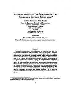
The Poisson race model has generally captured the relation between confidence and accuracy in the four experiments we have described. As discussed in the introduction, however, the model also has the ability to accommodate response times. This ability, which gives the model a major advantage over many other models of confidence calibration, has been ignored throughout the majority of this article. We now demonstrate the Poisson race model’s general ability to predict response times using the data of Experiments 1 and 2. Response times generally decrease as a function of confidence (Cartwright, 1941; Johnson, 1939; Kellogg, 1931), so it is important to examine whether the model can accommodate decreasing response times jointly with the calibration data.

0.55

0.65

0.75

0.85

0.95

Confidence

Figure 7. Fitted (dashed lines) and observed (solid lines) calibration, Experiment 4. The line with circles represents data from the easy condition, and the line with squares represents data from the hard condition. Error bars reflect standard errors of between-subjects variability in proportion correct.

For Experiments 1 and 2, observed and fitted response times are plotted as a function of confidence in Figure 8. The model predicted the decrease in mean response time with increased confidence, and it also picked up the mean difference between hard and easy conditions. It was more difficult to obtain an overall fit statistic here because the response times were continuous (as opposed to the proportions correct, which can be treated as categorical). To obtain an overall fit statistic, we first obtained a z statistic for each data point by subtracting each predicted response time from the corresponding observed response time and dividing by the observed standard error.10 Next, we squared each z statistic, which resulted in individual chi-square statistics with 1 degree of freedom. Finally, we summed the chi-square statistics and the degrees of freedom, and we subtracted the number of fitted model parameters from the degrees of freedom. This procedure resulted in a chi-square statistic of 82.39 with 18 degrees of freedom. This 9 Analytic expressions for response time predictions of the Poisson race model can be found in Townsend and Ashby (1983). 10 This procedure actually yielded a t statistic, but the degrees of freedom were always large enough to make it equivalent to a z statistic. Squared z statistics yield chi-square statistics, but squared t statistics do not.

POISSON RACE MODEL OF CONFIDENCE

1200 800

1000

RT (msec)

1400

1600

(a)

0.55

0.65

0.75

0.85

0.95

Confidence

403

extreme confidence judgment of 95%. The participant knows that 95% is the most extreme confidence judgment, and he or she has not sampled a large amount of information (in the model, extreme confidence judgments generally require the least amount of information). To be sure that 95% is the most appropriate confidence judgment for the stimulus, the participant samples some extra stimulus information. This would make the resulting response time similar to response times for 85% confidence judgments. More generally, the model is designed to handle problems of discrete choice or response selection. The model is not yet prepared to handle problems that require a person to provide an analog response as a result of some computations. Thus, this model cannot perform computation of a confidence interval (in the interval estimation task), and it cannot generate estimates of population and then a confidence associated with that estimate. The model cannot handle confidence-related processes from these tasks that carry over to confidence in discrete choice. Overall, we have demonstrated the model’s general ability to accommodate mean response time as a function of confidence. More complicated fit techniques involving the joint estimation of accuracy and response time will surely improve the model fits, along with modifications to critical model assumptions.

(b)

1200 800

1000

RT (msec)

1400

1600

General Discussion

0.55

0.65

0.75

0.85

0.95

Confidence

Figure 8. Fitted (dashed lines) and observed (solid lines) response time (RT) as a function of confidence, Experiments 1 and 2. The line with circles represents data from the easy condition, and the line with squares represents data from the hard condition. Error bars reflect standard errors of between-subjects variability in mean response time.

statistic generally reinforces the notion that the fits were less than adequate. Two weaknesses concerning the fits are the flattening of the observed mean response time functions for high confidence levels (Experiment 1; Figure 8A) and the overly rapid decrease of the predicted response time functions (Experiment 2; Figure 8B). These weaknesses likely reflect processes happening at the higher confidence levels that the model is not designed to explain, resulting in a mixture of processes. For example, imagine that, for a given experimental stimulus, a participant arrives at the most

In this article, we first reviewed both general findings in confidence calibration research and specific models geared toward explaining calibration data. Models under consideration include the decision variable partition model, the ecological model, and the class of error models. We noted shortcomings of these models, including the inability to account for some empirical findings, and we then presented the Poisson race model as an alternative to the other models. We conducted a series of general knowledge and perceptual categorization experiments to examine whether the Poisson race model can account for typical calibration data and to study the novel model prediction of response bias effects on calibration. We observed overconfidence and a hard– easy effect in our experiments, and the model successfully accommodated these findings. The model’s prediction of response bias effects was also supported by the data. Overall, our data are consistent with the Poisson race model. The Poisson race model has some advantages over other models of confidence. First, it describes a plausible process by which error enters into responses. Although such processes prove difficult to verify (e.g., Luce, 1995), the model may help us understand the psychological mechanisms underlying confidence elicitation. Furthermore, the fact that the Poisson race model depicts a psychological process gives its parameters convenient interpretations. For example, the setting of unequal threshold parameters in the model is interpreted as the introduction of response bias in an individual. Researchers may then experimentally induce response bias to examine the model’s performance. Compare this interpretation with the interpretation of, for instance, the decision variable partition model (Ferrell & McGoey, 1980). On the basis of a general signal detection model, the decision variable partition model yields confidence judgments via placement of partitions on the decision axis in a signal detection framework. One may elect to change the model’s partition parameters, which will, in turn, change the predicted confidence calibration. It is hypothesized that difficulty

404

MERKLE AND VAN ZANDT

manipulations cause partition parameters to be changed, but this is only because both difficulty manipulations and partition parameters have an effect on calibration. There is no psychological mechanism that explains why difficulty should cause a change in the partitions.

Calibration Mechanisms Given that parameters of the Poisson race model have a psychological interpretation, what exactly causes the model to produce overconfidence or underconfidence? In an attempt to answer this question, we explored the effects of individual model parameters on confidence calibration by systematically varying individual parameters while holding the others constant. It appears that the ␮ parameter (the discriminability between the high and low process) was the largest determinant of overconfidence magnitude and direction. When the ␮ parameter was large (for easily discriminable stimuli), the model tended to yield underconfidence. When the ␮ parameter was small (for indiscriminable stimuli), the model tended to yield overconfidence. Note that although the ␮ parameter has been characterized as representing discriminability, it may also be thought of as characterizing information quality. Thus, in a general knowledge context, ␮ would presumably vary with a decision maker’s quality of information for different alternatives. We can also explain the calibration differences under response bias predicted in Experiment 3. Our key assumption was that experimental response bias caused model thresholds to be unequal; the threshold for the favored alternative would be set less than the threshold for the unfavored alternative. As a result, an unfavored response would be made only if there was a large amount of evidence supporting the unfavored response and a small amount of evidence supporting the favored response. This leads to higher accuracy across the confidence range for unfavored responses as compared with favored responses. Thus, the accuracy difference contributes to greater overconfidence for favored responses as compared with unfavored responses.

Random Error in Confidence Judgments There has been some debate about the extent to which overconfidence and the hard– easy effect are due to random error instead of to cognitive biases. Erev et al. (1994) demonstrated that the perturbation of accurate confidence judgments by random error was enough to produce a standard overconfidence effect. Juslin et al. (2000) went on to claim that the hard– easy effect was a methodological artifact and that there was little evidence of cognitive bias as a contributor to overconfidence. Although we have discussed the hard– easy effect, we now make some clarification about random error in confidence judgments. Error exists in all models of confidence calibration. Models such as those used by Erev et al. (1994) specify pure random error, whereas models such as the Poisson race model specify a mechanism by which error enters into confidence judgments. One may therefore argue that, for all models under consideration, overconfidence arises as a result of error. Continuing with this viewpoint, models are simply vehicles by which error enters into confidence judgments. This view neglects the existence of cognitive biases: Error causes overconfidence, regardless of whether the error originates from purely random factors or from a cognitive bias. It is

therefore necessary to consider the locus of error and to avoid sweeping statements about overconfidence being due to error and not to cognitive biases. The specification and testing of process models of confidence provide a starting point for determining the nature of error. An example of a simple model that includes both a response error and a cognitive bias component comes from research on the better than average effect. Burson, Larrick, and Klayman (2006) presented a linear model of how people judge their own performance on experimental tasks in comparison with others. Overall error in the model is decomposed into error that arises from biases and error that arises randomly. Although this model was not fitted to data and was described as exploratory only, it may well be the case that confidence judgments (along with better than average judgments) are impacted by both cognitive bias and random error. The preceding discussion highlights the fact that current definitions of error and of cognitive biases are unclear. For the overconfidence phenomenon, a loose definition of cognitive bias might be “a mental mechanism causing people to think that they know more than they actually do know.” The fact that people are often overconfident cannot verify the existence of a cognitive overconfidence bias, and other explanations for overconfidence definitely exist. Erev et al.’s (1994) explanation was that of random error, whereas a second, related explanation is that people are simply not good at attaching a number to an internal feeling of confidence (e.g., Juslin, Olsson, & Bjo¨rkman, 1997). It is difficult to know where a cognitive bias ends and where random error begins. Each explanation assumes that bias or error occurs without the individual’s conscious awareness, and each explanation is capable of yielding overconfidence. With respect to the Poisson race model in particular, cognitive bias may be defined as “the inability to appropriately scale confidence judgments from stimulus information.” Because the Poisson race model yields overconfidence, such a definition supports the existence of a cognitive overconfidence bias in the Poisson race model. Although the cognitive overconfidence bias is usually described as “believing that one knows more than one actually does,” an alternative description might be “failing to appropriately modify one’s confidence judgments across varying difficult levels within a given task.” Confidence has been observed to change with proportion correct (Lindsay, Nilsen, & Read, 2000; Weber & Brewer, 2004), but the magnitude of change in confidence is often less than the magnitude of change in proportion correct. This suggests that people know when they know more and when they know less; they just do not know how to elicit confidence judgments that reflect their level of knowledge.

Conclusions The Poisson race model has accounted for classical confidence calibration effects, predicted a novel calibration effect, and shed light on factors giving rise to over- and underconfidence. The fact that the model also yields response time predictions means that the model has the potential to merge research on response times with research on confidence calibration. On a larger scale, the notion of a cognitive overconfidence bias has been explored in some detail. Mathematical modeling is an important tool that can help us define the term cognitive bias more specifically.

POISSON RACE MODEL OF CONFIDENCE

References Andrews, R. E. (2002, October 8). Message of the day. Retrieved October 8, 2002, from the U.S. House of Representatives Web site: http:// www.house.gov/andrews/welcome.htm Arkes, H. R., Dawson, N. V., Speroff, T., Harrell, F. E., Jr., Alzola, C., Phillips, R., et al. (1995). The covariance decomposition of the probability score and its use in evaluating prognostic estimates. Medical Decision Making, 15, 120 –131. Ashby, F. G., & Gott, R. E. (1988). Decision rules in the perception and categorization of multidimensional stimuli. Journal of Experimental Psychology: Learning, Memory, and Cognition, 14, 33–53. Baranski, J. V., & Petrusic, W. M. (1998). Probing the locus of confidence judgments: Experiments on the time to determine confidence. Journal of Experimental Psychology: Human Perception and Performance, 24, 929 –945. Baranski, J. V., & Petrusic, W. M. (1999). Realism of confidence in sensory discrimination. Perception & Psychophysics, 61, 1369 –1383. Barth, H., Kanwisher, N., & Spelke, E. (2003). The construction of large number representations in adults. Cognition, 86, 201–221. Bradfield, A. L., Wells, G. L., & Olson, E. A. (2002). The damaging effect of confirming feedback on the relation between eyewitness certainty and identification accuracy. Journal of Applied Psychology, 87, 112–120. Brewer, N., Keast, A., & Rishworth, A. (2002). The confidence–accuracy relationship in eyewitness identification: The effects of reflection and disconfirmation on correlation and calibration. Journal of Experimental Psychology: Applied, 8, 44 –56. Brunswik, E. (1955). Representative design and probabilistic theory in a functional psychology. Psychological Review, 62, 193–217. Burson, K. A., Larrick, R. P., & Klayman, J. (2006). Skilled or unskilled, but still unaware of it: How perceptions of difficulty drive miscalibration in relative comparisons. Journal of Personality and Social Psychology, 90, 60 –77. Cartwright, D. (1941). The relation of decision time to the categories of response. American Journal of Psychology, 54, 174 –196. Cohen, J. (1988). Statistical power analysis for the behavioral sciences (2nd ed.). Hillsdale, NJ: Erlbaum. Dawes, R. M. (1980). Confidence in intellectual vs. confidence in perceptual judgments. In E. D. Lantermann & H. Feger (Eds.), Similarity and choice: Papers in honor of Clyde Coombs (pp. 327–345). Bern, Switzerland: Han Huber. Dougherty, M. R. P. (2001). Integration of the ecological and error models of overconfidence using a multiple-trace memory model. Journal of Experimental Psychology: General, 130, 579 –599. Dunning, D., Heath, C., & Suls, J. M. (2004). Flawed self-assessment. Psychological Science in the Public Interest, 5, 69 –106. Erev, I., Wallsten, T. S., & Budescu, D. V. (1994). Simultaneous over- and underconfidence: The role of error in judgment processes. Psychological Review, 101, 519 –527. Espinoza-Varas, B., & Watson, C. (1993). Effects of decision criterion on latencies of binary decisions. Perception & Psychophysics, 55, 190 –203. Ferrell, W. R., & McGoey, P. J. (1980). A model of calibration for subjective probabilities. Organizational Behavior and Human Decision Processes, 26, 32–53. Gigerenzer, G., Hoffrage, U., & Kleinbo¨lting, H. (1991). Probabilistic mental models: A Brunswikian theory of confidence. Psychological Review, 98, 506 –528. Griffin, D., & Tversky, A. (1992). The weighing of evidence and the determinants of confidence. Cognitive Psychology, 24, 411– 435. Johnson, D. M. (1939). Confidence and speed in the two-category judgment. Archives of Psychology, 34, 1–53. Juslin, P., & Olsson, H. (1997). Thurstonian and Brunswikian origins of uncertainty in judgment: A sampling model of confidence in sensory discrimination. Psychological Review, 104, 344 –366. Juslin, P., Olsson, H., & Bjo¨rkman, M. (1997). Brunswikian and Thursto-

405

nian origins of bias in probability assessment: On the interpretation of stochastic components of judgment. Journal of Behavioral Decision Making, 10, 189 –209. Juslin, P., Olsson, N., & Winman, A. (1996). Calibration and diagnosticity of confidence in eyewitness identification: Comments on what can be inferred from the low confidence–accuracy correlation. Journal of Experimental Psychology: Learning, Memory, and Cognition, 22, 1304 – 1316. Juslin, P., Winman, A., & Olsson, H. (2000). Naive empiricism and dogmatism in confidence research: A critical examination of the hardeasy effect. Psychological Review, 107, 384 –396. Karlin, S. (1966). A first course in stochastic processes. New York: Academic Press. Kellogg, W. N. (1931). Time of judgment in psychometric measures. American Journal of Psychology, 43, 65– 86. Keren, G. (1988). On the ability of monitoring non-veridical perceptions and uncertain knowledge: Some calibration studies. Acta Psychologica, 67, 95–119. Keren, G. (1991). Calibration and probability judgments: Conceptual and methodological issues. Psychometrika, 77, 217–273. Klayman, J., Soll, J. B., Gonza´lez-Vallejo, C., & Barlas, S. (1999). Overconfidence: It depends on how, what, and whom you ask. Organizational Behavior and Human Decision Processes, 79, 216 –247. Koriat, A., & Goldsmith, M. (1996). Monitoring and control processes in the strategic regulation of memory accuracy. Psychological Review, 103, 490 –517. Koriat, A., Lichtenstein, S., & Fischhoff, B. (1980). Reasons for confidence. Journal of Experimental Psychology: Human Learning and Memory, 6, 107–118. Lee, W., & Janke, M. (1964). Categorizing externally distributed by stimulus samples for three continua. Journal of Experimental Psychology, 68, 376 –382. Leippe, M. R. (1980). Effects of integrative memorial and cognitive processes on the correspondence of eyewitness accuracy and confidence. Law and Human Behavior, 4, 261–274. Leippe, M. R. (1995). The case for expert testimony about eyewitness memory. Psychology, Public Policy, and Law, 1, 909 –959. Lichtenstein, S., & Fischhoff, B. (1977). Do those who know more also know more about how much they know? The calibration of probability judgments. Organizational Behavior and Human Performance, 20, 159 –183. Lichtenstein, S., Fischhoff, B., & Phillips, L. D. (1982). Calibration of probabilities: The state of the art to 1980. In D. Kahneman, P. Slovic, & A. Tversky (Eds.), Judgment under uncertainty: Heuristics and biases (pp. 306 –334). Cambridge, England: Cambridge University Press. Lindsay, D. S., Nilsen, E., & Read, J. D. (2000). Witnessing-condition heterogeneity and witnesses’ versus investigators’ confidence in the accuracy of witnesses’ identification decisions. Law and Human Behavior, 24, 685– 697. Luce, R. D. (1995). Four tensions concerning mathematical modeling in psychology. Annual Review of Psychology, 46, 1–26. Maddox, W. T., & Bohil, C. J. (2003). A theoretical framework for understanding the effects of simultaneous base-rate and payoff manipulations on decision criterion learning in perceptual categorization. Journal of Experimental Psychology: Learning, Memory, and Cognition, 29, 307–320. McKenzie, C. R. M. (1997). Underweighting alternatives and overconfidence. Organizational Behavior and Human Decision Processes, 71, 141–160. Olsson, H., & Winman, A. (1996). Underconfidence in sensory discrimination: The interaction between experimental setting and response strategies. Perception & Psychophysics, 58, 374 –382. Pike, R. (1971). The latencies of correct and incorrect responses in dis-

406

MERKLE AND VAN ZANDT

crimination and detection tasks: Their interpretation in terms of a model based on simple counting. Perception & Psychophysics, 9, 455– 460. Pike, R. (1973). Response latency models for signal detection. Psychological Review, 80, 53– 68. Pryke, S., Lindsay, R. C. L., Dysart, J. E., & Dupuis, P. (2004). Multiple independent identification decisions: A method of calibrating eyewitness identifications. Journal of Applied Psychology, 89, 73– 84. Ratcliff, R., & Smith, P. L. (2004). A comparison of sequential sampling models for two-choice reaction time. Psychological Review, 111, 333– 367. Ratcliff, R., Van Zandt, T., & McKoon, G. (1999). Comparing connectionist and diffusion models of reaction time. Psychological Review, 106, 261–300. Roberts, S., & Pashler, H. (2000). How persuasive is a good fit? Psychological Review, 107, 358 –367. Ronis, D. L., & Yates, J. F. (1987). Components of probability judgment accuracy: Individual consistency and effects of subject matter and assessment method. Organizational Behavior and Human Decision Processes, 40, 193–218. Rottenstreich, Y., & Tversky, A. (1997). Unpacking, repacking, and anchoring: Advances in support theory. Psychological Review, 104, 406 – 415. Rumelhart, D. E. (1970). A multicomponent theory of the perception of briefly exposed visual displays. Journal of Mathematical Psychology, 7, 191–218. Runeson, S., Juslin, P., & Olsson, H. (2000). Visual perception of dynamic properties: Cue heuristics versus direct-perceptual competence. Psychological Review, 107, 525–555. Schall, J. D. (2002). Decision-making: Neural correlates of response time. Current Biology, 12, R800 –R801. Schall, J. D. (2003). Neural correlates of decision processes: Neural and mental chronometry. Current Opinion in Neurobiology, 13(2), 182– 186. Smith, P. L., & Vickers, D. (1988). The accumulator model of two-choice discrimination. Journal of Mathematical Psychology, 32, 135–168. Sniezek, J. A., Paese, P. W., & Switzer, F. S., III. (1990). The effect of choosing on confidence in choice. Organizational Behavior and Human Decision Processes, 46, 264 –282.

Soll, J. B. (1996). Determinants of overconfidence and miscalibration: The roles of random error and ecological structure. Organizational Behavior and Human Decision Processes, 65, 117–137. Suantak, L., Bolger, F., & Ferrell, W. R. (1996). The hard-easy effect in subjective probability calibration. Organizational Behavior and Human Decision Processes, 67, 201–221. Taylor, H. M., & Karlin, S. (1998). An introduction to stochastic modeling (3rd ed.). Chestnut Hill, MA: Academic Press. Townsend, J. T., & Ashby, F. G. (1983). Stochastic modeling of elementary psychological processes. New York: Cambridge University Press. Van Zandt, T. (2000). ROC curves and confidence judgments in recognition memory. Journal of Experimental Psychology: Learning, Memory, and Cognition, 26, 582– 600. Van Zandt, T., & Maldonado-Molina, M. (2004). A mechanism for twochoice discrimination: Time-dependent response reversals in recognition memory. Journal of Experimental Psychology: Learning, Memory, and Cognition, 30, 1147–1166. Vickers, D. (1979). Decision processes in visual perception. New York: Academic Press. Vickers, D., & Pietsch, A. (2001). Decision making and memory: A critique of Juslin & Olsson’s (1997) sampling model of sensory discrimination. Psychological Review, 108, 789 – 804. Wallsten, T. S., & Budescu, D. V. (1983). Encoding subjective probabilities: A psychological and psychometric review. Management Science, 29, 152–173. Wallsten, T. S., & Gonza´lez-Vallejo, C. (1994). Statement verification: A stochastic model of judgment and response. Psychological Review, 101, 490 –504. Weber, N., & Brewer, N. (2004). Confidence–accuracy calibration in absolute and relative face recognition judgments. Journal of Experimental Psychology: Applied, 10, 156 –172. Wells, G. L. (1981). The tractability of eyewitness confidence and its implications for triers of fact. Journal of Applied Psychology, 66, 688 – 696. Yates, J. F., Lee, J.-W., & Bush, J. G. (1997). General knowledge overconfidence: Cross-national variations, response style, and “reality.” Organizational Behavior and Human Decision Processes, 70, 87–94.

Appendix Analytic Expressions of the Poisson Race Model In this appendix, we derive equations for the Poisson race model’s predictions of accuracy given a range of confidence. We first discuss the role that stimulus evidence plays in the model, and we then examine confidence and accuracy. Let N be a normally distributed stimulus evidence parameter favoring the high alternative (perceived numerosity), with mean ␮ and standard deviation ␴. The mean ␮ differs depending on whether the stimulus is actually high or low; when the stimulus is high, ␮ is large (positive), and when the stimulus is low, ␮ is small (negative). We must derive two information accumulation rates on the basis of N: one rate for information favoring the high alternative (␭H), and one rate for information favoring the low alternative (␭L). For mathematical simplicity and in accordance with Van Zandt (2000), we assume that the rates of information accumulation for the two alternatives sum to a constant, r. This means that we need only consider the density of ␭H ⫽ ␭, as ␭L ⫽ r ⫺ ␭. We can map N into the accumulation rate ␭ by the logistic transformation: ␭ ⫽ r/(1 ⫹ e⫺N). If N is large and positive, ␭ will be close to its maximum of r. If N is negative, ␭ will be closer to its minimum of 0. The probability density function of ␭ is given by (Van Zandt, 2000):

g共␭|␮,␴兲 ⫽

r ␭共r ⫺ ␭兲

冉 冉冋 冋 册 册 冊 冊

1

1 exp ⫺ 2 冑2␲␴

⫺ln

r⫺␭ ␭

2

⫺ ␮ /␴

,

(A1)

where both ␮ and ␴ may depend on whether the stimulus is high or low. For our analyses, we assumed that ␴ was the same for both high and low stimuli and that ␮L ⫽ ⫺␮H. It is useful to define a Bernoulli random variable, V, which represents the true stimulus identity. V equals 1 if the stimulus is high and 0 if the stimulus is low. The Bernoulli parameter P(V ⫽ 1) is equal to 0.5 because high and low stimuli are equally likely to occur on any given trial. We can then rewrite Equation A1 as g共␭|V ⫽ ␷) ⫽

r ␭(r ⫺ ␭)

1

冑2␲␴

冉 冉冋 冋 册 冉

exp ⫺

1 2

⫺ln

r⫺␭ ⫺ ␮H␷ ⫹ ␮L1⫺␷ ⫺ 1 ␭

冊册 冊 冊 2

/␴

.

(A2)

POISSON RACE MODEL OF CONFIDENCE

Confidence Predictions To derive the Poisson race model’s confidence predictions, we ultimately wish to find an expression for P(a ⱕ C ⬍ b, high wins | ␭) ⫽ fH(a,b | ␭), where C is the random variable representing confidence. That is, given some accumulation rate ␭, we wish to find the probability that confidence C for a high response falls in the range [a,b). Because confidence depends on the information accumulated on the counters at the time a response is made (see Equation 1), we can arrive at the probability of interest through the probability of losing counter states. If we restrict ourselves to responses in favor of high, the state Y of the losing counter (that of the low alternative) has a joint probability given by a negative binomial distribution (Townsend & Ashby, 1983; Van Zandt, 2000): P(Y ⫽ y, High wins) ⫽

冉

冊

KH ⫹ y ⫺ 1 KH p 共1 ⫺ p兲 y, y

(A3)

where KH is the threshold value of the high counter and p ⫽ ␭H/(␭H ⫹ ␭L) ⫽ ␭/r is the probability of an observer labeling a count as high. Continuing to restrict ourselves to high responses, we now examine the number of points on the losing counter that will yield confidence judgments between a and b. In other words, we transform the inequality involving C to an inequality involving Y:

冉 冉 冉

P(a ⱕ C ⬍ b, High wins) ⫽ P a ⱕ ⫽P ⫽P

冊 冊

KH ⬍ b, High wins KH ⫹ Y

Y 1 1 ⬍1⫹ ⱕ , High wins b KH a

冊

To obtain the joint probability for C when low wins, we (a) switch the H and L subscripts and (b) replace ␭/r with (r ⫺ ␭)/r both in Equation A4 and in the definitions for LB and UB.

Accuracy Predictions To generate calibration curves, we must compute the proportion of correct responses at a range of confidence between a and b: P(Correct | a ⱕ C ⬍ b). By definition, this probability may be rewritten as P(Correct, a ⱕ C ⬍ b) . P(a ⱕ C ⬍ b) Next, we use the law of total probability (Taylor & Karlin, 1998) to examine high responses (denoted “H” below) separately from low responses (denoted “L” below): P(Correct, a ⱕ C ⬍ b,“H”) ⫹ P共Correct, a ⱕ C ⬍ b, “L”) . P共a ⱕ C ⬍ b兲

冕

冊

册

⫽

⫽

冘冉

j⫽LB

冊冉 冊 冉 冊 KH

r⫺␭ j . r

P共a ⱕ C ⬍ b | ␭兲g共␭兲d␭.

0

冕

r

[ fH 共a,b | ␭兲 ⫹ fL 共a,b | ␭兲]g共␭兲d␭.

0

冘 1

g共␭兲 ⫽

1 g共␭ | V ⫽ ␷兲P共V ⫽ ␷兲 ⫽ 关g共␭ | V ⫽ 0兲 ⫹ g 共␭ | V ⫽ 1兲兴. 2 ␷⫽0

We can then write P(a ⱕ C ⬍ b)

fH共a,b | ␭兲 ⫽ P(a ⱕ C ⬍ b, High wins | ␭) ␭ r

r

We obtain the marginal density g(␭) by unconditioning Equation A2 over the value of V:

where ceil stands for the ceiling operator and floor stands for the floor operator. To obtain the probability of interest, we now use Equation A3 to sum over integers in the above inequality, giving

KH ⫹ j ⫺ 1 j

冕

[P共a ⱕ C ⬍ b,“H” | ␭兲 ⫹ P共a ⱕ C ⬍ b,“L” | ␭兲]g共␭兲d␭

0

KH ⫺ KH b KH ⫺ KH , KL ⫺ 1 , UB ⫽ min floor a

UB

P共a ⱕ C ⬍ b,␭兲d␭ ⫽

r

In this formula, the lower and upper bounds LB and UB take the following values:

冉 冊 冋 冉 冊

r

Applying the law of total probability again, we can expand the conditional probability P(a ⱕ C ⬍ b | ␭) to yield

KH KH ⫺ KH ⬍ Y ⱕ ⫺ KH, High wins ⫽ P共LB ⱕ Y ⱕ UB). P b a

LB ⫽ ceil

冕

0

KH KH ⫺ KH ⬍ Y ⱕ ⫺ KH , for 0 ⱕ Y ⬍ KL. b a

冉

(A5)

The three probabilities in Equation A5 are derived separately below. The denominator probability P(a ⱕ C ⬍ b) is a function of fH(a,b | ␭) and fL(a,b | ␭). We first use the law of total probability to express P(a ⱕ C ⬍ b) after integrating over all values of ␭, so

P共a ⱕ C ⬍ b兲 ⫽

The restriction that 0 ⱕ Y ⬍ KL incorporates the (joint) event that the high counter wins, meaning that the low counter must have fewer than KL counts. As a result, we can modify the joint probability as

407

(A4)

This probability is conditioned on the threshold values KH and KL. Although we do not explicitly note it here for simplicity, this fact becomes important when variable thresholds are specified later.

⫽

1 2

冕

r

关fH 共a,b | ␭兲 ⫹ fL 共a,b | ␭兲兴关g共␭ | V ⫽ 0兲 ⫹ g共␭ | V ⫽ 1兲兴d␭.

(A6)

0

Note that Equation A6 can be used to estimate the confidence distribution; that is, it gives the marginal probability that confidence is observed at a given level.

(Appendix continues)

MERKLE AND VAN ZANDT

408

P(Correct | a ⱕ C ⬍ b)P(Correct | a ⱕ C ⬍ b)

Next, we consider the first term in Equation A5, the probability of a correct high response with confidence between a and b. Using the Bernoulli variable V, ⫽

P(Correct, a ⱕ C ⬍ b, “H”) ⫽ P共V ⫽ 1, a ⱕ C ⬍ b, “H”兲.

冕

冕

r

[fH 共a,b | ␭兲g共␭|V ⫽ 1兲 ⫹ fL共a,b | ␭兲g共␭ | V ⫽ 0兲] d␭

0

.

r

(A9)

关fH 共a,b | ␭兲 ⫹ fL共a,b | ␭兲兴关g共␭ | V ⫽ 0兲 ⫹ g共␭ | V ⫽ 1兲兴 d␭

0

We now follow the same steps as in the derivation of Equation A6:

冉

冊 冕冉 r

P V ⫽ 1, a ⱕ C ⬍ b, “H” ⫽

冕

r

P共a ⱕ C ⬍ b, “H”, ␭ | V ⫽ 1兲P共V ⫽ 1兲d␭

冕

1 ⫽ 2 1 2

冊

P V ⫽ 1, a ⱕ C ⬍ b, “H”, ␭ d␭

0

0

⫽

⫽

Variable Thresholds

冕

P(Correct | a ⱕ C ⬍ b) ⫽

r

P共a ⱕ C ⬍ b, “H”, ␭ | V ⫽ 1兲d␭

0

⫽

r

P共a ⱕ C ⬍ b, “H” | ␭,V ⫽ 1兲g共␭ | V ⫽ 1兲d␭

0

⫽

As we have alluded to, Equation A9 is implicitly conditioned on the threshold parameters KH and KL being equal to constants. If the threshold parameters have probability distributions associated with them, then we must account for these distributions in the expression for P(Correct | a ⱕ C ⬍ b). We rewrite P(Correct | a ⱕ C ⬍ b) in the following manner:

1 2

冕

⫽

r

P共a ⱕ C ⬍ b, “H” | ␭兲g共␭ | V ⫽ 1兲d␭

0

⫽

1 2

冕

fH 共a,b | ␭兲g共␭ | V ⫽ 1兲d␭.

(A7)

冕

(A8)

0

Similarly, 1 2

r

fL共a,b | ␭兲g共␭ | V ⫽ 0兲d␭.

⌺ kP共Correct, a ⱕ C ⬍ b, K ⫽ k兲 ⌺ kP共a ⱕ C ⬍ b | K ⫽ k兲P共K ⫽ k兲

⌺ kP共Correct | a ⱕ C ⬍ b, K ⫽ k兲P共a ⱕ C ⬍ b | K ⫽ k兲P共K ⫽ k兲 , ⌺ kP共a ⱕ C ⬍ b | K ⫽ k兲P共K ⫽ k兲 (A10)

r

P(Correct, a ⱕ C ⬍ b, “L”) ⫽

P共Correct, a ⱕ C ⬍ b兲 P共a ⱕ C ⬍ b兲

0

We arrive at a final formula for the calibration curve by substituting Equations A6, A7, and A8 into Equation A5 (note that the factor 1/2 cancels):

where K is a vector containing the two threshold parameters. These steps follow by definition of conditional probabilities. The probability P(Correct | a ⱕ C ⬍ b, K ⫽ k) is given by Equation A9, the probability P(a ⱕ C ⬍ b | K ⫽ k) is given by Equation A6, and the probability P(K ⫽ k) is set by the experimenter. Intuitively, Equation A10 is simply a weighted average of proportions correct P(Correct | a ⱕ C ⬍ b, KH ⫽ i, KL ⫽ j) across all possible threshold combinations. The weights are determined by both the probability that each threshold combination occurs P(K ⫽ k) ⫽ P(KH ⫽ i, KL ⫽ j) and the probability that confidence falls in the range [a,b) under a certain threshold combination P(a ⱕ C ⬍ b | KH ⫽ i, KL ⫽ j).

Received October 28, 2004 Revision received March 7, 2006 Accepted March 13, 2006 䡲