An open-source application to model and solve dynamic fault tree of real industrial ...... [10] J.B. Dugan, J.S. Bavuso, M.A Boyd, âDynamic fault-tree models for.
1
An open-source application to model and solve dynamic fault tree of real industrial systems Ferdinando Chiacchio1, Lucio Compagno2, Diego D’Urso2, Gabriele Manno1 and Natalia Trapani2 1
2
Dipartimento di Matematica e Informatica, Università degli Studi di Catania (ITALY) Dipartimento di Ingegneria Industriale e Meccanica, Università degli Studi di Catania (ITALY)
In recent years, a new generation of modeling tools for the risk assessment have been developed. The concept of “dynamic” was exported also in the field of reliability and techniques like dynamic fault tree, dynamic reliability block diagrams, boolean logic driven Markov processes, etc., have become of use. But, despite the promises of researchers and the efforts of end-users, the dynamic paradox hangs: risk assessment procedures are not as straight as they were with the traditional static methods and, what is worse, it is difficult to assess the reliability of these results. Far from deny the importance of the scientific achievement, we have tested and cursed some of these dynamic tools realizing that none of them was appropriate to solve a real case. In this context, we decided to develop a new DFT reliability solver, based on the Monte Carlo simulative approach. The tool is greatly powerful because it is written with Matlab® code, hence is open-source and can be extended. In this first version, we have implemented the most used dynamic gates (PAND, SEQ, FDEP and SPARE), the existence of repeated events and the possibility to simulate different cumulative distribution function of failure (Weibull, negative exponential CDF and constant). The tool is provided with a snappy graphic user interface written in Java®, which allows an easy but efficient modeling of any fault tree schema. The tool has been tested with many literature cases of study and results encourage other developments. Index Terms— Reliability, Dynamic Fault Tree, Monte Carlo simulation, Parallel Computing, Continuous time Markov chains.
I.
I
INTRODUCTION
n recent years the importance of risk assessment in the industrial field has significantly increased and the most used tools of RAMS – the well known combinatorial techniques such as Reliability Block Diagram (RBD) and Static Fault Tree (SFT) – have been object of a reasonable criticism. In fact, these techniques are not able to model the timedependent behaviors of a system (or a process), like the replacement of spare components, a chain of events and so on. State-space models have been used in order to overcome the previous limits and, on the wave of their success, other formalisms were proposed, such as: • DFT (Dynamic Fault Tree) [1]; • DRBD (Dynamic Reliability Block Diagrams) [2]; • BDMP (Boolean logic Driven Markov Process) [3]. The declared aim was to combine the intutive symbolic representation of the combinatorial methods with the powerful modeling of the state space models: these new techniques were named “dynamic” and, conversely, the combinatorial ones were referred as “static”. Among these new formalisms, the dynamic fault tree analysis (DFT) has been one of the most promising [4] because, with the introduction of the dynamic gates, the power of the modeling increases but the effort of the designing is kept low (like in static fault tree). The reason of our interest in this technique is that most of the risk assessments in the industrial field are still based on the static fault tree, hence a re-examination of such risk reports with the aid of the DFT could be a valuable work. The attempt to apply the DFT technique to some existing reliability schema typical of the industrial field is discussed in [5], where the inadequacy of the traditional analytical methods is shown for complex systems, the limits of the most known automated software of reliability are highlighted and the lines for the development of a simulative algorithm in a spreadsheet environment are traced (ie. Excel®).
Starting from the results [5], in this paper we present a software tool for the resolution of complex DFT model, based on the direct Monte Carlo simulative approach [6]. The paper is organized as follow: in the second section we introduce the DFT technique, briefly mentioning the resolution procedures and the limits of the most used tools; in the third paragraph we describe the simulative approach for the fault tree resolution and in the fourth we introduce our Monte Carlo engine (MatCarloRE), implemented within the Matlab® framework; in the fifth paragraph, the Java® graphic user interface (GUI) (jDFTDes, which stands for java Dynamic Fault Tree Designer) that embeds the MatCarloRE library is presented and in the sixth section some results are discussed and compared with the enhancing of the parallel computing approach. In the end conclusion are drawn. II.
THE DYNAMIC FAULT TREE TECHNIQUE
A Dynamic Fault Tree (DFT) is a stochastic model for the reliability evaluation that synthesizes the ways how an undesired and time dependent event can occur. As a Static Fault Tree (SFT), a DFT is composed by a top gate which represents the most undesired event (TE, top event) and a certain number of lower level gates and basic events (BEs) that, combined according with the logic of the fault scenario, cause the occurrence of the TE. The main hypotheses for the use of the DFT are that (i) events are binary and (ii), according to many authors [7-9], components are not repairable. Thus, the main difference with the SFT is that DFT were not conceived to compute the availability but are appropriate to evaluate the reliability of model characterized by complex stochastic dependencies (Fig. 1). The possibility to model complex interactions with the graphical symbolism of the SFT has encouraged the development of dynamic models [10] but, in point of the fact, DFT has shown many issues for what concern their resolution.
2 The reason of this anomaly has to be traced in the lack of a rigorous semantic language [11] that has caused the proliferation of several and variegated techniques of resolution that resort to an equivalent stochastic model [1, 11-13]. At the state of the art, an analytical solution exists only if another hypothesis is added to the previous ones [9]: BEs have to be described by the exponential distribution. In this way, it is possible to convert a DFT into a state-space model and solve it within the domain of the Markov processes. Unfortunately the mentioned hypotheses can result too restrictive, especially for real industrial applications characterized not only by exponentially distributed time to fail but also by Weibull, gaussian or lognormal probability distribution. Therefore, the reliability evaluation of systems that present generalized functions of probability is not possible with the analytical Markov processes and, at the state of the art, the more effective solution is the simulation [14, 15].
Fig. 1: the most frequently used dynamic gates
In general, all the previous techniques of resolution (analytical and simulative) have been implemented in a lot of software applications for reliability analysis [16, 17] but, despite that, the real effectiveness of these tools is still questionable because none of them can be used to design and solve “complex DFT” in a straightforward manner. In Table 1, we synthesize the main features of some automated tools that we have tested; for more details about their characteristics we remind to [5]. Table 1: main features of the reliability automated tools for DFT TOOL MAIN RESULTS LIMITS RELEX
Reliability Availability Importance Measures
Results are questionable NO nested dynamic gates Only exponential CDF
GALILEO
Reliability Sensitivity
NO repeated events
BDMP
Reliability Availability Importance Measures and Sensitivity
Not intuitive (introducing other formalism)
In our scope, a “complex DFT" is a model that presents a combination of the following characteristics: repeated events, events characterized by generalized distributions of probability and nested dynamic gates. All of these elements are necessary to obtain an accurate modeling of the failure scenarios in real industrial systems. III.
MONTE CARLO SIMULATION IN RELIABILITY ASSESSMENT
Monte Carlo simulation is a statistical method used to solve real problems in many engineering field, in particular when analytical approaches are not feasible. This method is based on the generation of a large number of realizations of the simulated process, which represent the generic random walk inside a discrete “phase space” of the system configurations. In this method, a certain number of stochastic sampling (called iterations, runs or batches of the simulation) of the independent variables are performed in order to implement the simulated process; for this reason, a Monte Carlo simulation cannot produce an exact evaluation as it is computed as a weighted average among the results of the generated phase space. Nowadays, this class of methods is gaining a lot of interest due to the power of modern computers that permit to speed up the simulative process and collect a large number of runs, ensuring higher accuracy. For reliability evaluations [18, 19], the main advantage of the simulative approach over the analytical ones is that it is possible to remove the hypothesis of the exponential distribution and, more in general, to implement any kind of failure and safety logic. The other important difference concerns the resolution process: with the simulative paradigma the computation of a TE needs the information from the entire parts of the fault tree (ie. single components and sub-models), whereas the analytical solutions mix these dynamics in a set of ordinary differential equations. Hence, at the end of a simulation it is possible to retrieve also information about the other parts of the fault tree (BEs and intermediate events), whereas with the analytical methods this would need an ad-hoc computation for the sub-system of interest. In our approach, we make use of the direct Monte Carlo simulation [6] that considers BEs as single entities, sampling the time of failure of any BE once, at the beginning of any iteration. These information are used to evaluate the logic of the gates which the BEs are connected with, in order to retrieve the state and the trigger time of each gate. In turn, these information are passed to the gates of the higher levels, ascending the fault tree up to the TE gate. From the implementation point of view, the main advantage of this approach is the modularity, as the algorithms behind the logic of the gates (static and dynamic) can be implemented separately. In order to build up a Monte Carlo simulation, let us consider the following notation:
3 1) FT is the generic fault tree composed by a number n of BEs; at the beginning of any iteration, the method will sample n stochastic time of failure tfi, one for each BEi; 2) F(t) is the unreliability of the system at the time t, computed as the probability that the system is down at the time t, F(t) = P(system is down); 3) S = (s1, s2,..,sn) is the generic “vector of the states” where si represents the state of the i-th component that can be ‘working (=0) or ‘failed’ (=1) and represents a point of the phase space of the system; 4) Φ is the set of all the vectors of the states S in which the system fails and depends on the structure of the fault tree; 5) Hk={S(t0); S(t1);...; S(Tm)} is the evolution of the k-th iteration of the Monte Carlo simulation; in general, the evolution Hk of an iteration can be characterized by a number of different vectors of the states S; in fact, these vectors are determined with respect to the stochastic times of failure generated at the beginning of the Monte Carlo sampling. For instance, let consider the simple SFT of Fig. 2 and assume a Monte Carlo simulation of K iterations and a mission time Tm = 10h. In this case Φ = {(1A, 1B, 1C)}, no matter the sequences of failures of the components.
Fig. 2: a simple example of SFT and DFT
Now, let us consider the generic i-th iteration (i