an application of time series arima forecasting model for predicting ...

Studies in Business and Economics

AN APPLICATION OF TIME SERIES ARIMA FORECASTING MODEL FOR PREDICTING SUGARCANE PRODUCTION IN INDIA

KUMAR Manoj Victoria University College, Yangon, Myanmar ANAND Madhu Agra University, UP, India Abstract: A time series modeling approach (Box-Jenkins’ ARIMA model) has been used in this study to forecast sugarcane production in India. The order of the best ARIMA model was found to be (2,1,0). Further, efforts were made to forecast, as accurate as possible, the future sugarcane production for a period upto five years by fitting ARIMA(2,1,0) model to our time series data. The forecast results have shown that the annual sugarcane production will grow in 2013, then will take a sharp dip in 2014 and in subsequent years 2015 through 2017, it will continuously grow with an average growth rate of approximately 3% year-on-year.

Key words: forecasting, time series modeling, ARIMA, sugarcane production, India

1. Introduction India, known as the original home of sugar, is the world’s second largest producer (as on 2012) of sugarcane next only to Brazil. After textile industry, the sugar industry, with around Rs. 300 billions (= $5 billion, as on date $1 = INR60 approx.) of turnover, is the second largest among the agro-based processing industries in India. Table 1 below represents the 62 years’ sugarcane production in India. The data is taken from the secondary source, Department of Agriculture and Cooperation (DAC) in India, from 1950 to 2012. In this paper, an effort is made to forecast sugarcane production for the five leading years. The model developed for forecasting is an Autoregressive Integrated Moving Average (ARIMA) model. This model was introduced by Box and Jenkins in 1960 and hence this model is also known as Box-Jenkins Model which is used to forecast a single variable. The main reason of choosing ARIMA model in this study for the forecasting is because this model assumes and takes into account the non-zero autocorrelation between the successive values of the time series data.

Studies in Business and Economics - 81 -

Studies in Business and Economics The open source statistical software ‘R’ (build 3.0.1) and various statistical and time series packages such as ‘tseries, ‘fUnitRoots’, ‘forecast’ and ‘TTR’ etc are used along with other standard packages for this study purpose. Table 1: Sugarcane Production in India (in Millions of Tons) Sl No

Year

Production

Sl No

Year

Production

Sl No

Year

Production

1 1950-51

57.05

22 1971-72

113.57

43

1992-93

228.04

2 1951-52

61.63

23 1972-73

124.87

44

1993-94

229.66

3 1952-53

51.00

24 1973-74

140.81

45

1994-95

275.54

4 1953-54

44.41

25 1974-75

144.29

46

1995-96

281.10

5 1954-55

58.74

26 1975-76

140.60

47

1996-97

277.56

6 1955-56

60.54

27 1976-77

153.01

48

1997-98

279.55

7 1956-57

69.05

28 1977-78

176.97

49

1998-99

288.73

8 1957-58

71.16

29 1978-79

151.66

50

1999-00

299.33

9 1958-59

73.36

30 1979-80

128.83

51

2000-01

295.96

10 1959-60

77.82

31 1980-81

154.25

52

2001-02

298.43

11 1960-61

110.00

32 1981-82

186.36

53

2002-03

281.58

12 1961-62

103.97

33 1982-83

189.51

54

2003-04

233.87

13 1962-63

91.91

34 1983-84

174.08

55

2004-05

237.09

14 1963-64

104.23

35 1984-85

170.32

56

2005-06

281.18

15 1964-65

121.91

36 1985-86

170.65

57

2006-07

355.52

16 1965-66

123.99

37 1986-87

186.09

58

2007-08

348.19

17 1966-67

92.83

38 1987-88

196.74

59

2008-09

285.03

18 1967-68

95.50

39 1988-89

203.04

60

2009-10

292.31

19 1968-69

124.68

40 1989-90

225.57

61

2010-11

339.17

20 1969-70

135.02

41 1990-91

241.05

62

2011-12

342.20

21 1970-71

126.37

42 1991-92

254.00

Source: Department of Agriculture and Cooperation, India 2. Literature Review Raymond Y.C. Tse, (1997) suggested that the following two questions must be answered to identify the data series in a time series analysis: (1) whether the data are random; and (2) have any trends? This is followed by another three steps of model identification, parameter estimation and testing for model validity. If a series is random, the correlation between successive values in a time series is close to zero. If the

- 82 - Studies in Business and Economics

Studies in Business and Economics observations of time series are statistically dependent on each another, then the ARIMA is appropriate for the time series analysis. Meyler et al (1998) drew a framework for ARIMA time series models for forecasting Irish inflation. In their research, they emphasized heavily on optimizing forecast performance while focusing more on minimizing out-of-sample forecast errors rather than maximizing in-sample ‘goodness of fit’. Stergiou (1989) in his research used ARIMA model technique on a 17 years' time series data (from 1964 to 1980 and 204 observations) of monthly catches of pilchard (Sardina pilchardus) from Greek waters for forecasting up to 12 months ahead and forecasts were compared with actual data for 1981 which was not used in the estimation of the parameters. The research found mean error as 14% suggesting that ARIMA procedure was capable of forecasting the complex dynamics of the Greek pilchard fishery, which, otherwise, was difficult to predict because of the year-to-year changes in oceanographic and biological conditions. Contreras et al (2003) in their study, using ARIMA methodology, provided a method to predict next-day electricity prices both for spot markets and long-term contracts for mainland Spain and Californian markets. In fact a plethora of research studies is available to justify that a careful and precise selection of ARIMA model can be fitted to the time series data of single variable (with any kind of pattern in the series and with autocorrelations between the successive values in the time series) to forecast, with better accuracy, the future values in the series. This study is also an attempt to predict the future production values of sugarcane in India by fitting ARIMA technique on the time series data of past 62 years’ productions. 3. Box-Jenkins (ARIMA) Model: Basics A time series is defined as a sequence of data observed over time. ARIMA models are a class of models that have capabilities to represent stationary as well as non-stationary time series and to produce accurate forecasts based on a description of historical data of single variable. Since it does not assume any particular pattern in the historical data of the time series that is to be forecast, this model is very different from other models used for forecasting. The approach of Box-Jenkins methodology in order to build ARIMA models is based on the following steps: (1) Model Identification, (2) Parameter Estimation and Selection, (3) Diagnostic Checking (or Modal Validation); and (4) Model's use. Model identification involves determining the orders (p, d, and q) of the AR and MA components of the model. Basically it seeks the answers for whether data is stationary or non-stationary? What is the order of differentiation (d), which makes the time stationary?

Studies in Business and Economics - 83 -

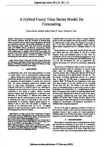
Studies in Business and Economics 4. Time Series Analysis and Building ARIMA The given set of data in Table 1 is used to develop forecasting model. The Picture 1 below represents the line plot of sugarcane production in India.

Figure 1: Sugarcane Production (Million Tonnes) in India from 1951 to 2012 Since we already have discussed that to build an ARIMA model for forecasting of a variable requires following steps: 1) Model Identification, (2) Parameter Estimation and Selection, and (3) Diagnostic Checking (or Modal Validation); before we can (4) use the Model for forecasting application. We, therefore, will first try to identify the model for fitness. 5. Model Identification First stage of ARIMA model building is to identify whether the variable, which is being forecasted, is stationary in time series or not. By stationary we mean, the values of variable over time varies around a constant mean and variance. The time plot of the sugarcane production data in Picture 1 above clearly shows that the data is not stationary (actually, it shows an increasing trend in time series). The ARIMA model cannot be built until we make this series stationary. We first have to difference the time series ‘d’ times to obtain a stationary series in order to have an ARIMA(p,d,q) model with ‘d’ as the order of differencing used. Caution to be taken in differencing as overdifferencing will tend to increase in the standard deviation, rather than a reduction. The best idea is to start with differencing with lowest order (of first order, d=1) and test the data for unit root problems. So we obtained a time series of first order differencing and Figure 2 below is the line plot of the first order differenced sugarcane production data.

- 84 - Studies in Business and Economics

Studies in Business and Economics

Figure 2: Line plot of differenced sugarcane production data of first order (d=1) It can easily be inferred from the above graph (Picture 2) that the time series appears to be stationary both in its mean and variance. But before moving further, we will first test the differenced time series data for stationary (unit root problem) using augmented Dickey-Fuller test.

6. Test for stationarity: Augmented Dickey-Fuller (ADF) Test Our null hypothesis (H0) in the test is that the time series data is non-stationary while alternative hypothesis (Ha) is that the series is stationary. The hypothesis then is th tested by performing appropriate differencing of the data in d order and applying the ADF test to the differenced time series data. First order differencing (d=1) means we generate a table of differenced data of current and immediate previous one (Xt = Xt – Xt-1). The ADF test result, as obtained upon application, is shown below: Dickey-Fuller = -5.5395, Lag order = 3, p-value = 0.01 We, therefore, fail to accept the H0 and hence can conclude that the alternative hypothesis is true i.e. the series is stationary in its mean and variance. Thus, there is no need for further differencing the time series and we adopt d = 1 for our ARIMA(p,d,q) model. This test enables us to go further in steps for ARIMA model development i.e. to find suitable values of p in AR and q in MA in our model. For that, we need to examine the correlogram and partial correlogram of the stationary (first order differenced) time series.

Studies in Business and Economics - 85 -

Studies in Business and Economics

7. Correlogram and Partial Correlogram The Figure 3 below represents the plot of correlogram (auto-correlation function, ACF) for lags 1 to 20 of the first order differenced time series of the sugarcane production in India.

Figure 3: Autocorrelations (ACF) of first differenced series by lag The above correlogram infers that the auto-correlation at lag 1 does not exceed the significance limits and auto-correlations tail off to zero after lag 3. Although the autocorrelation at lag 5 just exceeds the significant limits (ACF coefficient at lag 5 = 0.336), rest all coefficients between lag 4 and 20 are well within the limits. We can assume that lag 5 autocorrelation is an error and happened by chance alone. The Figure 4 below represents the partial correlogram (partial auto-correlation function, PACF) for lags 1 to 20 of the differenced time series.

Figure 4: Partial Autocorrelations (PACF) of first differenced series by lag

- 86 - Studies in Business and Economics

Studies in Business and Economics The partial correlogram, above in Figure 4, also infers that partial autocorrelation coefficient does not exceed significant limits at lag 1 and after lag 2 partial autocorrelation tails off to zero. Although here also we have one outlier at lag 7 (coefficient at lag 7 is almost touching the significant limits), which we can assume that it is an error and happened due to by chance alone because all the other PACFs from lag 3 to 20 are within the significant limits. The Table 2 below represents the ACF and PACF coefficients for lag 1 to 20 of that first order differenced series. Table 2: ACF and PACF Coefficients for lag 1 to 20 Lag

ACF

PACF

Lag

ACF

PACF

1

0.202

0.202

11

-0.07

-0.1

2

-0.62

-0.685

12

0.132

-0.02

3

-0.4

-0.094

13

0.091

-0.11

4

0.213

-0.122

14

-0.15

-0.16

5

0.336

-0.046

15

-0.14

-0.04

6

-0.05

-0.155

16

0.087

-0.02

7

-0.11

0.249

17

0.176

-0.01

8

0.017

-0.095

18

-0.01

0.011

9

-0.02

0.008

19

-0.09

0.138

10

-0.1

-0.103

20

0.021

0.034

Since the correlogram (ACF) tailing off to zero after lag 3 (omitting the outlier) and the partial correlogram (PACF) tailing off to zero after lag 2 (omitting the outlier), we can define the following possible ARMA (auto regressive moving average) models for the first differenced time series data of sugarcane production in India: 1. An ARMA(2,0) model i.e. autoregressive model of order p=2 since the partial autocorrelation is zero after lag 2 and the autocorrelation is zero. 2. An ARMA(0,3) model i.e. moving average model of order q=3 since the autocorrelation is zero after lag 3 and the partial autocorrelation is zero. 3. An ARMA(p,q) model i.e. a mix model with p and q both greater than 0 since autocorrelation and partial autocorrelation both tail off to zero. 8. Selecting the candidate model for forecasting Since ARMA(2,0) has 2 parameters in it, ARMA(0,3) has 3 parameters in it and ARMA(p,q) has at least 2 parameters in it, therefore, by using principle of parsimony, the models ARMA(2,0) and ARMA(p,q) are the best candidate models for further step. In the next step, we have to device the best ARIMA model using the ARMA(2,0) model (with p=2 & q=0), ARMA(p,q) mixed model (with p & q both greater

Studies in Business and Economics - 87 -

Studies in Business and Economics than 0), and order of differencing . Therefore, based upon the conditions, we can have only following three tentative ARIMA(p,d,q) models: ARIMA(p,d,q): ARIMA(2,1,0), ARIMA(2,1,1), and ARIMA(2,1,2) To select as the best suitable model for forecasting out of three above, we will choose the one with lowest BIC (Bayesian Information Criterion) and AIC (Akaike Information Criterion) values. Following Table 3 summarizes the output of each of the fitted ARIMA model in our time series (of sugarcane production data): Table 3: AIC and BIC values of fitted ARIMA models ARIMA Model

Coefficients AR1

AR2

MA1

σ MA2

2

Log

AIC

BIC

AICc

(Est) Liklihood

(2,1,0) 0.3783 -0.6652

265.4

-257.39

520.78 527.11 521.2

(2,1,1) 0.3733 -0.6639 0.0088

265.3

-257.39

522.77 531.22 523.49

(2,1,2) 0.3518 -0.7594 0.0118 0.1754 262.1

-257.06

524.12 534.68 525.21

We can clearly observe in the table above that the lowest AIC and BIC values are for the ARIMA(2,1,0) model with (p=2, d=1 and q=0) and hence this model can be the best predictive model for making forecasts for future values of our time series data. 9. Forecasting using selected ARIMA model The above selected model ARIMA(2,1,0), which we are fitting to our time series data, means that we are fitting ARMA(2,0) model of first order difference to our time series. Also, ARMA(2,0) model, which has two parameters in it, can be rewritten an AR model of order 2, or AR(2) model, since q is zero in MA. Therefore, this model can be expressed as: Xt = µ + (β1 * (Zt-1 - µ)) + (β2 * (Zt-2 - µ)) + εt, Where Xt is the stationary time series we are studying, µ is the mean of time series Xt, β1 and β2 are parameters to be estimated (the AR1 and AR2 terms in the fitted ARIMA(2,1,0) model values as above in Table 3, i.e. AR1 = 0.3783 and AR2= 0.6652), and εt is white noise with mean zero and constant variance. One caution here, as a standard for a stationary differenced time series, the mean (µ) should be either equal or very close to zero. If µ is not zero (as in our case it is 5.13), we use the value of the mean in the above equation for forecasting the future values. We now will fit the chosen ARIMA(2,1,0) model to forecast for the future values of our time series. Following Table 4 shows the forecast for the next 5 years with 80%, 95% and 99.5% (low and high) prediction intervals:

- 88 - Studies in Business and Economics

Studies in Business and Economics Table 4: 5-Year Forecasting for Sugarcane Production Prediction Forecast Low 80 High 80 Low 95 High 95 Low 99.5 High 99.5 2013

350.489 329.614 371.365 318.563 382.416

304.764

396.215

2014

322.601 287.053 358.149 268.235 376.967

244.739

400.463

2015

325.031 285.243 364.818 264.181 385.881

237.882

412.179

2016

344.502 303.817 385.187 282.28 406.724

255.388

433.615

2017

350.25

257.216

443.285

307.776 392.725 285.291 415.21

Figure 5 and Figure 6 below show the plot for 5 years’ forecast of the sugarcane production by fitting ARIMA(2,1,0) model to our time series data:

Figure 5: Forecasts from ARIMA(2,1,0) In the picture above, the two shaded zones of forecast represent the 80% and 95% (lower and upper side) projection of prediction intervals.

Figure 6: Forecast fitted with ARIMA(2,1,0)

Studies in Business and Economics - 89 -

Studies in Business and Economics The Figure 6 above shows the fitted ARIMA(2,1,0) along with upper control limit and lower control limit of forecast. Next, we will investigate (1) the forecast errors of our ARIMA(2,1,0) model, whether or not these are normally distributed with mean zero and constant variance; (2) whether there are any correlations between successive forecast errors; and (3) if residuals are white noise. To investigate distribution of forecasting errors, we will plot the errors (standard residuals). Pictures 6(a), 6(b), 6(c), 6(d) and 6(e) below show various plots and histograms of standard residuals (forecast errors) of fitted ARIMA(2,1,0) model:

Figure 6 (a): Plot of Standard residual of fitted ARIMA(2,1,0)

Figure 6 (b): Plot of Residuals (Forecast Errors) – ARIMA(2,1,0)

- 90 - Studies in Business and Economics

Studies in Business and Economics

Figure 6 (c): Histogram of Forecast Errors (Residuals) – ARIMA(2,1,0)

Figure 6 (d): Histogram of Residuals (Forecast Errors) – ARIMA(2,1,0)

Figure 6 (e): Normal Q-Q Plot of Residuals (Forecast Errors) – ARIMA(2,1,0)

Studies in Business and Economics - 91 -

Studies in Business and Economics The careful investigation from the various line plots and Q-Q plot of standard residuals in the fitted model (above in Picture 6(a) and 6(b)) infers that standard errors are roughly constant in its mean and variance overtime (although there seems to be some higher variance towards the end of the time series i.e. in the most recent decade). This is confirmed by the histograms of the residuals as well (Picture 7(c) and 7(d)). The two histograms (of the errors’ distribution) above infer that the errors are (almost) normally distributed and mean of the distribution seems to be zero. The Q-Q plot in Picture 7 (e) also seems to confirm the normality in errors. To investigate further whether there are any correlations between successive forecast errors, we will plot the correlogram (ACF) and partial correlogram (PACF) of the forecast errors. Following Pictures 7(a) and 7(b) represents ACF and PACF of the forecast errors:

Figure 7(a): Estimated ACF of Residuals (Forecast Errors) – ARIMA(2,1,0) It is clearly evident from the ACF plot above that none of the autocorrelation coefficients between lag 1 and 20 are breaching the significant limits i.e. all the ACF values are well within the significant bounds.

Figure 7(b): Estimated PACF of Residuals – ARIMA(2,1,0)

- 92 - Studies in Business and Economics

Studies in Business and Economics Similarly ACFs, all the PACFs or partial autocorrelation coefficients of residuals of fitted ARIMA for lag 1 to lag 10 are within the significant limits. This means ACF and PACF concluded that there is no non-zero autocorrelations in the forecast residuals (or standard errors) at lag 1 to 20 in the fitted ARIMA(2,1,0) model. The Box-Ljung test results are shown in the Table 5 below shows the Box-Ljung and Box-Pierce test statistics while Picture 8 below represents the plot of Box-Ljung p-values for the fitted model: Table 5: Box-Ljung and Box-Pierce Test Statistics 2 Test X Deg. Of Freedom p-value Box-Ljung 17.6672 20 0.6093 Box-Pierce 14.8789 20 0.7832

Figure 7: Plot of Ljung-Box p-values of fitted ARIMA(2,1,0) The statistics and large p-values in both the tests above is suggesting us to accept the null hypothesis that all of the autocorrelation functions in lag 1 to 20 are zero. In other words, we can conclude that there is no (or almost nil) evidence for non-zero autocorrelations in the forecast errors at lags 1 to 20 in our fitted model. 10. Conclusions In this study, the ARIMA(2,1,0) was the best candidate model selected for making predictions for upto 5 years for the production of sugarcane in India using a 62 years' time series data. ARIMA was used for the reasons of its capabilities to make predictions using a time series data with any kind of pattern and with autocorrelations between the successive values in the time series. The study also statistically tested and validated that the successive residuals (forecast errors) in the fitted ARIMA time series were not correlated, and the residuals seem to be normally distributed with mean zero and constant variance. Hence, we can conclude that the selected

Studies in Business and Economics - 93 -

Studies in Business and Economics ARIMA(2,1,0) seem to provide an adequate predictive model for the sugarcane production in India. The ARIMA(2,1,0) model predicted an increase in the production for year 2013, then a fall in 2014 and in subsequent year upto 2017, overall an increase in production (Table 5). The prediction for 2013 is resulted approximately 350 million tons (±6% at confidence interval 80%, ±9% at confidence interval 95% and ±13% at confidence interval 99.5%) and for 2014, the prediction is approximately 322 million tons (±11% at confidence interval 80%, ±17% at confidence interval 95% and ±24% at confidence interval 99.5%). Although, like any other predictive models in forecasting, ARIMA also has limitations on accuracy of predictions yet it is used more widely for forecasting the future successive values in the time series. 11. References Coghlan, Avril (2010), A Little Book of R for Time Series, Readthedocs.org, Available online at: http://a-little-book-of-r-for-time-series.readthedocs.org/en/latest/src/timeseries.html Contreras, J., Espinola, R., Nogales, F.J., Conejo, A.J., (2003), ARIMA Models to Predict Nextday Electricity Prices, IEEE Transactions on Power Systems, Vol. 18, No. 3, pp. 10141020. Hannan, E., (1980), The Estimation of the Order of ARMA Process, Annals of Statistics, Vol. 8, pp. 1071-1081. Jeffrey E. J., (1990), Evaluating Methods for Forecasting Earnings Per Share, Managerial Finance, Vol. 16, No. 3, pp. 30–35. Ljung, G.M. and Box, G.E.P. (1978), On a measure of lack of fit in time series models, Biometrika, Vol. 67, pp. 297-303. Meyler, Aidan; Kenny, Geoff and Quinn, Terry (1998), Forecasting Irish inflation using ARIMA models, Central Bank and Financial Services Authority of Ireland Technical Paper Series, Vol. 1998, No. 3/RT/98 (December 1998), pp. 1-48. Raymond Y.C. Tse (1997), An application of the ARIMA model to real-estate prices in Hong Kong, Journal of Property Finance, Vol. 8, No. 2, pp.152 – 163. Stergiou, K. I. (1989), Modeling and forecasting the fishery for pilchard (Sardina pilchardus) in Greek waters using ARIMA time-series models, ICES Journal of Marine Science, Volume 46, No. 1, Pp. 16-23.

- 94 - Studies in Business and Economics