An approach for developing numeric nutrient criteria ...

EPA/600/R-08/004 January 2008

An Approach for Developing Numeric Nutrient Criteria for a Gulf Coast Estuary Contributing Authors James D. Hagy III, Ph.D. Research Ecologist U.S. Environmental Protection Agency Office of Research and Development National Health and Environmental Effects Research Laboratory Gulf Ecology Division Gulf Breeze, FL Janis C. Kurtz, Ph.D. Research Ecologist U.S. Environmental Protection Agency Office of Research and Development National Health and Environmental Effects Research Laboratory Gulf Ecology Division Gulf Breeze, FL Richard M. Greene, Ph.D. Branch Chief, Ecological Dynamics and Effects Branch U.S. Environmental Protection Agency Office of Research and Development National Health and Environmental Effects Research Laboratory Gulf Ecology Division Gulf Breeze, FL

U.S. Environmental Protection Agency Office of Research and Development National Health and Environmental Effects Research Laboratory Gulf Ecology Division 1 Sabine Island Drive, Gulf Breeze, FL 32561

Disclaimer This report provides information to States, Indian tribes (hereafter tribes), and other authorized jurisdictions for the purpose of assisting development of numeric nutrient criteria for adoption into water quality standards under the Clean Water Act (CWA). Under the CWA, States and tribes are to establish water quality criteria to protect designated uses. State and tribal decisionmakers retain the discretion to adopt approaches on a case-by-case basis that differ from the approaches used in this report when appropriate and scientifically defensible. Although this report provides hypothetical numeric nutrient criteria that would serve to protect resource quality and aquatic life, it does not substitute for the CWA or U.S. Environmental Protection Agency’s (EPA’s) regulations nor is it a regulation itself. Thus, it cannot impose legally binding requirements on EPA, States, tribes, or the regulated community and may not apply to a particular situation or circumstance.

Citation Hagy, J. D., J. C. Kurtz, and R. M. Greene. 2008. An approach for developing numeric nutrient criteria for a Gulf coast estuary. U.S. Environmental Protection Agency, Office of Research and Development, National Health and Environmental Effects Research Laboratory, Research Triangle Park, NC. EPA 600R-08/004. 44 pp.

Cover photo by James Hagy ii

Table of Contents List of Tables ...........................................................................................................................................iv List of Figures...........................................................................................................................................v Executive Summary............................................................................................................................. vii 1. Introduction.........................................................................................................................................1 1.1 Background .....................................................................................................................................1 1.2 Study Site ........................................................................................................................................3 2. Methods ...............................................................................................................................................7 2.1 Water Quality Data for Pensacola Bay ...........................................................................................7 2.2 Ecoregional Water Quality Characterization ..................................................................................7 2.3 Aerial Submerged Aquatic Vegetation Surveys .............................................................................8 2.4 Watershed Characteristics and Land Use........................................................................................9 3. Results and Discussion .....................................................................................................................11 3.1 Ecoregional Comparisons and the Percentile Approach...............................................................11 3.2 Algal Biomass, Productivity, and Community Composition........................................................14 3.3 Preventing Hypoxia.......................................................................................................................16 3.4 Protecting Seagrass Habitats .........................................................................................................18 3.5 A Watershed Perspective ..............................................................................................................20 3.6 Nutrient Criteria ............................................................................................................................22 4. Summary and Conclusions...............................................................................................................27 5. References..........................................................................................................................................29 Appendix A: Observations in EPA’s Level III Ecoregion 75 ................................................................33 Appendix B: Observations in Florida’s Level IV Ecoregion 75a...........................................................34 Appendix C: List of Acronyms and Abbreviations ................................................................................35

iii

List of Tables Table 1. Sources of water quality data used in this study.........................................................................7 Table 2. Ecoregional water quality conditions computed for U.S. Environmental Protection Agency’s Level III ecoregion 75 and Florida’s Level IV ecoregion 75a ...............................................14 Table 3. Seasonal median chlorophyll-a in Pensacola Bay surface waters and its interquartile range...................................................................................................................................15 Table 4. Plankton community respiration rate and sediment oxygen demand in the Pensacola Bay system .....................................................................................................................................................17 Table 5. Area of submerged aquatic vegetation beds in the Pensacola Bay system circa 1950 and in 1960, 1980, 1992, and 2003................................................................................................19 Table 6. Suggested nutrient and nutrient-related water quality criteria for Pensacola Bay resulting from the weight-of-evidence approach described herein.........................................................25

iv

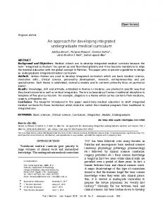
List of Figures Figure 1. Locations of stations sampled during two major studies of water quality conditions in the Pensacola Bay system and a 2003-to-2004 study of benthic and planktonic metabolism .............3 Figure 2. A conceptual model illustrating historic, ecologic, and socioeconomic factors of potential importance for developing and evaluating water quality management options for Pensacola Bay...........................................................................................................................................4 Figure 3. The locations of water quality monitoring stations visited under the Environmental Monitoring and Assessment Program during 2001 and 2002 and the Florida Inshore Monitoring and Assessment Program during 2000 through 2004 ...............................................................................8 Figure 4. Procedure for computing statistical comparison values for estuaries .......................................8 Figure 5. Distribution of summer estuary median surface water quality values by salinity zones for estuaries in Level III ecoregion 75 and Level IV ecoregion 75a ......................................................13 Figure 6. Frequency histogram of surface chlorophyll-a concentrations in mesohaline waters of the Pensacola Bay system from 1996 to 2001....................................................................................15 Figure 7. Observations of bottom dissolved oxygen in the Pensacola Bay system during the summers of 1996 through 1999 indicating the locations and frequency of observations less than 2.0 mg L-1................................................................................................................................................16 Figure 8. Coverage of submersed aquatic vegetation in Pensacola Bay circa 1950 and in 1992...........18 Figure 9. Land cover in the Pensacola Bay watershed circa 2001 .........................................................21 Figure 10. Flow diagram illustrating the logical path followed to determine an appropriate approach for determining nutrient criteria for Pensacola Bay ...............................................................................23

v

Acknowledgments This manuscript would not have been possible without the vision and sustained efforts of a large number of people at the Gulf Ecology Division, whose work over more than a decade provided much of the data available to characterize water quality and ecological processes in Pensacola Bay. Much of this work has been published separately and cited herein. We thank Mike Lewis and Richard Devereux for sharing unpublished data and Linda Harwell for assistance in obtaining data from the National Coastal Assessment and Florida's Inshore Monitoring and Assessment Program. Ed Decker helped us better understand how regulatory mechanisms function under the Clean Water Act. Ed Dettman, Walt Nelson, and Cheryl Brown provided helpful comments at several stages of manuscript preparation. We appreciate the significant contributions of several individuals who edited the document and developed its final layout. These include John Barton and Keith Tarpley of NHEERL's National Information Management and Site Support Staff and Barbra Schwartz and others at the National Center for Environmental Assessment. This is contribution no.1322 of the Gulf Ecology Division of the U.S. Environmental Protection Agency’s National Health and Environmental Effects Research Laboratory.

vi

Executive Summary compared with water quality within corresponding salinity zones in other estuaries. Chlorophyll-a in Pensacola Bay was comparable with the median for ecoregion 75 and was somewhat higher than other systems in ecoregion 75a. Nutrients and water clarity in oligohaline water were also similar to the median. In contrast, water clarity and nutrient concentrations in mesohaline and higher salinity waters were in the best 25% of estuaries (>75th percentile for water clarity and 18). We defined each estuary according to the boundaries of estuarine drainage areas (EDAs) defined by the National Ocean and Atmospheric Administration's Coastal Assessment Framework (NOAA 1999a). Data from IMAP and NCA were referenced to EDAs within the coastal assessment framework using a geographic information

All Water Quality Observations in the Class during Summer

Oligohaline Zone (Surface Salinity18)

Medians by Estuary

25th or 75th Percentile

Figure 4. Procedure for computing statistical comparison values for estuaries. The 25th percentile of estuary medians was used for comparison values for water quality indicators where lower values are better (e.g., nutrients, chlorophyll-a). The 75th percentile was used for secchi depth, where higher values indicate higher water clarity.

8

(Homer et al. 2004; http://www.mrlc.gov/). The database provides land use and land cover classifications at 30-m resolution. Classifications are derived from Landsat-7 Enhanced Thematic Mapper imagery and additional supporting data. Land cover data for the Pensacola Bay watershed were extracted from the larger data set and tabulated by classification using the ArcGIS 9.2 geographic information system indicated above.

coverage data for 2003 were obtained from the USGS National Wetlands Research Center, Lafayette, LA.

2.4 Watershed Characteristics and Land Use Data describing land use in the Pensacola Bay watershed were obtained from the 2001 National Land Cover Database using the MultiResolution Land Cover Consortium Viewer

9

10

3. Results and Discussion encompasses much of the coast surrounding Pensacola Bay and a significant span of coastline mostly to the east of the bay (Figure 3). Although the definition of these ecoregions is based on climatological, geological, and biological attributes (Omernik 1987) and pertains to the watersheds of estuaries rather than to the estuaries themselves, we expect that the ecological character of inshore coastal waters must reflect to some degree the ecological attributes of the surrounding land. Moreover, because the ecoregions define geographically contiguous regions of the coast, we expect similarity in many attributes to arise simply from proximity. Important differences can occur, however, particularly when the ecoregion spans oceanographically distinct regions. For example, tides vary dramatically within ecoregion 75; minimal diurnal tides occur on the northern Gulf coast, whereas large semidiurnal tides occur along the Atlantic coast of Georgia and South Carolina. These differences alone contribute to other large ecological differences, such as the presence of extensive intertidal salt marshes in Georgia (Dame et al. 2000), which practically define the Georgia coast, versus the more limited extent of salt marshes in west Florida. The smaller spatial extent of Florida’s Level IV ecoregions eliminates the most glaring withinclass differences, but at the cost of a class that includes fewer systems. Even though it is likely that important differences remain within even these smaller classes, further division leads toward the perspective that every estuary is completely unique, precluding any role for comparative ecological analysis in development of nutrient criteria. U.S. EPA (2000a,b) define a variety of options for determining reference conditions for classes of freshwater systems. The preferred approach is to derive water quality criteria on the basis of conditions in relatively pristine water bodies. When a set of sufficiently pristine water

3.1 Ecoregional Comparisons and the Percentile Approach Identifying appropriate benchmarks or “reference conditions” against which to compare water quality conditions is a key feature of EPA’s recommended approaches for developing nutrient criteria (U.S. EPA 2000a,b). We modified EPA’s percentile approach for freshwaters to define benchmark water quality values that have potential applicability to Pensacola Bay. A central feature of the approach, which we applied here, is identification of a suitable class of similar estuaries from which a reference condition can be determined. In the context of nutrients, similarity refers to a similarity in ecological attributes that influence the response of a system to nutrient inputs. There are many classification schemes for coastal systems, each serving different objectives and emphasizing different ecological attributes (Kurtz et al. 2006). Unfortunately, there is little consensus regarding which classification schemes would be most appropriate in terms of predicting response to nutrient inputs. None have been demonstrated to be useful for that purpose. One concern is that, even though many important attributes of estuaries have been considered (e.g., residence time, mean depth, ratio of watershed area to estuary area; Kurtz et al. 2006), a much broader set of factors (e.g., climate, geology, character of offshore water quality) likely contributes to the ecological character of ecosystems. As an alternative to the available estuarine classifications, we utilized EPA’s Level III ecoregions and, simultaneously, the more finely resolved Level IV ecoregions for Florida to define a class of estuaries for Pensacola Bay. Pensacola Bay lies within the “southern coastal plain” ecoregion 75 in the Level III scheme (Figure 3). The shores of Pensacola Bay include several of Florida’s Level IV ecoregions, but the “Gulf coastal flatwoods region” (ecoregion 75a) 11

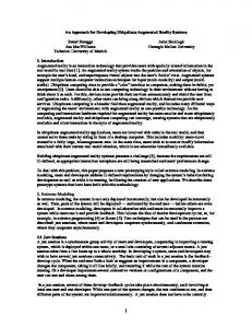
several important ways. First, because the available regional-scale data sets from NCA and IMAP include only late summer data (Table 1), our analysis is limited to summer (June through September). We do not see this as a major limitation because most water quality problems related to nutrient enrichment, especially hypoxia, are expressed primarily during summer. Thus, we assumed that, if water quality supports the designated uses during summer, uses outside of summer are also likely to be met. The second difference is that we divided observations into salinity zones, based on the principle that water quality parameters in estuaries commonly vary along the salinity gradient. We selected three zones (salinity < 5, 5-18, and > 18) with the objective of resolving differences associated with the salinity gradient, while ensuring that a sufficient quantity of data was available in each zone in most estuaries. Our objectives in defining the zones likely could have been met with different definitions (i.e., breakpoints); however, an attempt to define values for a greater number of salinity zones likely would have resulted in excessive parsing of the available data. Finally, we consider the values obtained via this approach to be guidelines or comparison values, not values that can be adopted defensibly as criteria without further scientific support. The computed median values show that summer water quality in a significant portion of estuaries in ecoregions 75 and 75a was characterized by low nutrient and moderate chlorophyll-a concentrations, with concentrations generally lower in ecoregion 75a than in ecoregion 75 as a whole (Figure 5, Table 2). Concentrations of chlorophyll-a, nitrogen, and phosphorus are commonly higher in Mid-Atlantic estuaries (NOAA 1997). Nutrient concentrations are commonly higher in Pacific coast estuaries influenced by coastal upwelling (NOAA 1998). Summer median nutrient concentrations and water clarity in Pensacola Bay were comparable to or lower than the 25th percentile (higher than the 75th percentile for water clarity) for the ecoregion, with a few exceptions.

bodies can be identified, criteria have been based on the 75th percentile of water body median values for such pristine sites (U.S. EPA 2000a,b). Given the pervasive human presence in many coastal marine areas, we assumed that few, if any, estuaries were sufficiently pristine to adapt this approach for estuaries. Another approach is a historical reference condition in which water quality conditions observed prior to significant anthropogenic impacts provide a basis for comparison. For most estuaries, limited availability of historical data precludes this approach. The record of historical water quality data for Pensacola Bay is unusually extensive, but, as is common, early monitoring was undertaken in response to obvious pollution impacts (Olinger et al. 1975) and does not quantify the unimpaired or pristine condition. Thus, historical data cannot be used to characterize pristine water quality conditions in Pensacola Bay. Lacking either pristine sites or adequate historical data, we derived levels we call “comparison values” from the statistical distribution of water quality conditions in all the estuaries in the class (Figure 4), adapting the percentile approach of U.S. EPA (2000a,b). Because the class includes sites subject to a range of nutrient enrichment, we utilized the 25th percentile of estuary median water quality values to derive comparison values. EPA (2000a,b) cite empirical evidence from lakes to support this choice when reference quality sites are not available. We did not assume that there is any relationship between the 25th percentile of estuary median water quality and water quality in a hypothetical set of pristine estuaries. We simply chose to examine the 25th percentile as a potentially useful reference point in the distribution of estuary medians. For water clarity, the same ideas apply, but higher values indicate “better” water quality. Therefore, we used the 75th percentile as a comparison value. We contrasted values based on two classes: (1) all estuaries in ecoregion 75 (Appendix A) and (2) the subset of those estuaries within ecoregion 75a (Appendix B). Our application of the percentile approach differs from that of U.S. EPA (2000a,b) in 12

Bay than the 25th percentile values in all salinity zones for both ecoregion 75 and ecoregion 75a (Table 2). Instead, median chlorophyll-a in Pensacola Bay was similar to the median for ecoregion 75 and closer to the upper quartile for ecoregion 75a (Figure 5). The statistical approach described here is a repeatable, quantitative scheme for computing water quality measures that can serve as comparison values for both causal variables (e.g., nutrients) and nutrient-related response variables such as water clarity (secchi depth) and chlorophyll-a. In the absence of water quality thresholds clearly tied to loss of ecological integrity, these comparison values are useful for placing values Figure 5. Distribution of summer estuary median surface water quality values by for any one estuary in salinity zones for estuaries in Level III ecoregion 75 (left three plots) and Level IV perspective. There are ecoregion 75a (right three plots). Salinity zones are oligohaline (O; salinity < 5), mesohaline (M; salinity 5-18)], polyhaline (P; salinity > 18). Red lines indicate summer several factors that limit medians by salinity zone for Pensacola Bay. Identical values are shown in both the left the range of + and right halves of each plot. DIN = NO2 + NO3 + NH4 ; TN = total nitrogen, TP = total interpretations for these phosphorus. comparison values. One question is whether the 25th percentile (or 75th Inorganic nitrogen and phosphorus percentile for water clarity) of estuary medians is concentrations in oligohaline waters were higher an appropriate comparison value, and whether it than the 25th percentile, but concentrations in approximates a minimum condition protective of higher salinity water were comparable or lower designated uses as suggested by EPA (2000a,b). than the corresponding 25th percentile in those A broader comparison with the distribution of salinity zones. Total phosphorus (TP) values in the ecoregion (i.e., Figure 5) gives a concentrations were comparable to the 25th more complete comparative perspective but still percentile values across the salinity zones, leaves open the question of whether a particular whereas total nitrogen (TN) concentrations were water quality value supports use attainment. comparatively lower in oligohaline waters and Water quality values at the 25th percentile of the higher in polyhaline waters (Figure 5, Table 2). ecoregional distribution could be either Median chlorophyll-a was higher in Pensacola 13

Table 2. Ecoregional water quality conditions for chlorophyll-a (Chl-a), secchi depth, dissolved inorganic + 3nitrogen (DIN = NO2 + NO3 + NH4 ), phosphate (PO4 ), total nitrogen (TN), and total phosphorus (TP) computed for EPA’s Level III ecoregion 75 and Florida’s Level IV ecoregion 75a. Values are the 25th percentile of summer estuary medians, except for secchi depth, where the value is the 75th percentile of estuary medians. Summer medians for Pensacola Bay are shown for comparison. Data are for surface water. Values in parentheses for ecoregion 75 and 75a are the number of estuaries included for each variable. Values in parentheses for Pensacola Bay are the number of observations included. TN and TP values were not computed for ecoregion 75 because data were only available for a portion of the ecoregion. Pensacola Bay medians were computed from a combined data set that includes EPA’s EMAP quarterly surveys (1996 to 2001, EPA’s monthly surveys (2002 to 2004), and Florida’s IMAP surveys. IMAP sampled Pensacola Bay intensively in 2003 and also visited two stations in 2004.

Group

Chl-a (µg l-1)

Secchi Depth (m)

DIN (µM)

3-

PO4 (µM)

TN (µM)

TP (µM)

Oligohaline (Salinity < 5) Ecoregion 75 Ecoregion 75a Pensacola Bay

3.8 (16) 2.1 (6) 5.6 (103)

0.93 (12) 1.6 (4) 0.9 (93)

2.9 (15) 2.6 (6) 8.7 (102)

0.11 (15) 0.023 (6) 0.18 (86)

nd 23.4 (6) 29.2 (49)

nd 0.67 (6) 0.88 (32)

Mesohaline (Salinity 5-18) Ecoregion 75 Ecoregion 75a Pensacola Bay

5.1 (21) 4.1 (7) 7.3 (233)

1.0 (21) 1.0 (7) 1.2 (198)

1.3 (20) 0.81 (7) 0.97 (210)

0.13 (21) 0.065 (7) 0.11 (122)

nd 26.5 (7) 31.7 (59)

nd 0.56 (7) 0.55 (47)

4.3 (28) 3.5 (6) 5.8 (107)

1.3 (28) 1.4 (5) 2.0 (100)

0.59 (27) 0.47 (6) 0.44 (102)

0.11 (28) 0.052 (6) 0.048 (82)

nd 20.5 (6) 32.7 (57)

nd 0.73 (6) 0.43 (56)

Polyhaline (Salinity > 18) Ecoregion 75 Ecoregion 75a Pensacola Bay nd = No data

and eutrophication in aquatic systems, obvious reasons why it already is used widely in water quality management related to nutrients. Other simple descriptors of the phytoplankton community, such as productivity; community composition, including presence of harmful algae; and growth dynamics, also can provide useful insights. We assembled basic information about the phytoplankton community in Pensacola Bay to explore its implications, if any, for managing nutrients in the bay. Seasonal and salinity zone chlorophyll-a medians varied between 1.6 and 7.4 μg L-1, with the highest values during summer (5.6 to 7.3 μg L-1; Table 3). Both summer and nonsummer values were “low” to “medium” according to standard ranges described by NOAA (1997). “High” concentrations (>20 μg L-1) occurred very infrequently (Table 3, Figure 6). Of 1,390 chlorophyll-a measurements in the Pensacola Bay system between 1996 and 2004, only 36 (2.5%) were greater than 20 μg L-1. Murrell et al. (2007) measured phytoplankton production rates in Escambia Bay using carbon

nonprotective of uses or excessively restrictive for a particular estuary. A second concern is the assumption that the estuaries in either ecoregion 75 or ecoregion 75a are an appropriate “class,” and that Pensacola Bay is a member of that class. We suggest that the percentile approach is likely to produce values in a reasonable range for estuaries, but that, because the approach is inherently independent from effects-based considerations and is not certain to generate appropriate values, the values should be evaluated in the context of other information available about the estuary in question before they could be used to determine criteria. In the following sections, we discuss ecological conditions and processes in the Pensacola Bay system to provide a thorough evaluation of the science that may be pertinent to selection of numeric nutrient criteria.

3.2 Algal Biomass, Productivity, and Community Composition Chlorophyll-a is an easily monitored and conceptually appealing indicator of trophic status 14

Table 3. Seasonal median chlorophyll-a in Pensacola Bay surface waters and its interquartile range (25th to 75th percentile). Salinity zones were determined from surface water salinity. Median Chlorophyll-a -1 (μg L )

The available information points to several key conclusions regarding the phytoplankton community in Pensacola Bay. First, there is no clear evidence that the phytoplankton community is stimulated strongly by excess nutrients, or that it is unbalanced or otherwise causing adverse ecological effects. If chlorophyll-a concentrations were frequently in NOAA’s (1997) high (20 to 60 μg L-1) or “hypereutrophic” (>60 μg L-1) range, or, if annual phytoplankton productivity was among the highest found in estuaries, one might have a priori cause for concern regarding excess phytoplankton. Median summer chlorophyll-a concentrations were generally higher than the 25th percentile of systems within the ecoregion, especially for ecoregion 75a (Table 2). However, the small differences are probably not ecologically significant. We do not know of any study directly implicating chlorophyll-a concentrations in the low range observed in Pensacola Bay with failure to support any human or aquatic life uses. Experimental evidence (Murrell et al. 2002, Juhl and Murrell 2005) shows that phytoplankton biomass and production in Pensacola Bay are limited by nutrients. This provides a mechanistic expectation that increased nutrient inputs will

Interquartile Range (μg L-1)

Oligohaline (Salinity < 5) Winter 2.2 Spring 4.0 Summer 5.6 Fall 1.6 Mesohaline (Salinity 5-18) Winter 3.5 Spring 5.8 Summer 7.3 Fall 5.0 Polyhaline (Salinity > 18) Winter 3.4 Spring 3.8 Summer 5.8 Fall 3.4

(1.2 - 3.7) (2.6 - 5.4) (3.8 - 8.7) (1.2 - 3.7) (2.6 - 5.2) (3.7 - 8.4) (5.1 - 10.7) (3.1 - 7.2) (2.6 - 4.7) (2.1 - 4.8) (3.8 - 8.1) (2.5 - 6.0)

14 uptake methods and estimated that annual phytoplankton productivity was 320 g carbon m-2 year-1 (0.88 g carbon m-2 day-1). Among estuaries, where annual production commonly varies between 100 and 500 g carbon m-2 year-1 (Boynton et al. 1982, Boynton and Kemp 2007), the annual production rate for Pensacola Bay is “mesotrophic” or moderate. The summer phytoplankton assemblage is dominated by cyanobacteria (Murrell and Lores 2004, Murrell and Caffrey 2005), whose low chlorophyll-a content relative to carbon (phycoerythrin is the dominant light-gathering pigment in most cyanobacteria; MacIntyre et al. 2002) undoubtedly contributes to the high ratio of annual productivity to chlorophyll-a. The phytoplankton community in Pensacola Bay is usually nutrient limited and can be limited by either phosphorus or nitrogen (Murrell et al. 2002, Juhl and Murrell 2005). Relief of nutrient limitation associated with periods of increased freshwater and nutrient inputs manifests as increased Figure 6. Frequency histogram of surface chlorophyll-a chlorophyll-a concentration, increased concentrations in mesohaline (surface salinity = 5-18) waters of the Pensacola Bay system from 1996 to 2001. “Low,” “Medium,” phytoplankton production (Murrell et al. and “High” designations refer to descriptors used by NOAA 2007), and a greater relative abundance of (1997). Dotted lines indicate the median concentration. Data are eukaryotic phytoplankton (Juhl and Murrell from the EPA/ORD quarterly surveys of Pensacola Bay. 2005) in Pensacola Bay. 15

phytoplankton, we expect that increased nutrient inputs would increase phytoplankton production and biomass in Pensacola Bay.

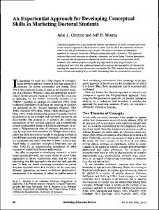
3.3 Preventing Hypoxia Hypoxia, which we define here as DO < 2 mg L-1, is a common phenomenon in bottom waters of Pensacola Bay (Hagy and Murrell 2007). Where it occurs, hypoxia should be a concern because of its direct impact on marine life (Diaz and Rosenberg 1995). Globally, hypoxia has increased in coastal waters in some relation to nutrient overenrichment, commonly causing negative effects on the health and productivity of biological communities (Diaz 2001). Thus, hypoxia is a significant threat to both human (e.g., fisheries) and aquatic life use attainment in coastal systems. Observations of hypoxia in the Pensacola Bay system date back to Hopkins (1969), who found oxygen concentrations as low as 0.48 mg L-1 in bottom waters of Escambia Bay during a late-summer study. Olinger et al. (1975) reported bottom water oxygen less than 1 mg L-1 in Escambia Bay but concluded that conditions had improved since 1969. The recent monthly survey data (Table 1) show that hypoxic bottom waters occurred between April and November, with the maximum extent in late summer (Figure 7). Hypoxia currently affects an average of 25% of the bay bottom during summer and can, at times, affect a much larger fraction (Figure 7). Olinger et al. (1975) recognized long ago that the bay often was strongly stratified, and that weak circulation probably contributed to the risk of hypoxia. Hagy and Murrell (2007) quantified the stratification and circulation to better characterize conditions that create a high susceptibility to hypoxia. They found that hypoxia developed in Pensacola Bay despite moderate oxygen consumption rates in the lower water column and sediments. Total (i.e., combined) oxygen consumption for the lower water column and sediments was estimated to be 0 to 1.5 g oxygen m-2 day-1 using a box model (Hagy and Murrell 2007). The model estimates were in reasonable agreement with average integrated oxygen consumption rates (0.94 g oxygen m-2 day-1) measured during summer at

Figure 7. Observations of bottom dissolved oxygen in the Pensacola Bay system during the summers of 1996 through 1999 indicating the locations and frequency of observations less than 2.0 mg L-1, a level commonly used as an operational definition of hypoxia. Data are from EPA/ORD quarterly surveys (upper panels). The computed extent of hypoxia in Pensacola Bay by month from 2002 to 2004, based on EPA/ORD monthly transect surveys (lower panel).

increase phytoplankton production and possibly phytoplankton biomass. Unfortunately, simple linear dose-response relationships fail to capture the relationship between nutrient loads or concentrations and chlorophyll-a in Pensacola Bay (Murrell et al. 2007). Relationships that we expect to observe on the basis of known causal mechanisms often are hidden by the natural complexity that characterizes estuarine ecosystems (e.g., flushing, food web interactions) and, therefore, are not easily seen in field observations (Cloern 2001). Some empirical relationships between nutrients and chlorophyll-a have been found among systems and, through time, within systems (Boynton et al. 1982); however, such relationships usually are only adequate to provide broad direction for management (i.e., increased nutrients are associated with higher chlorophyll-a). Nonetheless, it is important and useful to recognize that, on the basis of experimental evidence documenting nutrient limitation of 16

direct effects of hypoxia on many species of marine life are known (Diaz and Rosenburg 1995, Campbell and Goodman 2004). Although current science for Pensacola Bay cannot predict the magnitude of increase in extent or severity of hypoxia expected from a particular increase in nutrient inputs or the extent to which the severity of hypoxia might increase, both conceptual and quantitative models indicate that increased nutrients most likely would increase the extent and severity of hypoxia, resulting in loss of existing aquatic life uses. Defining a broadly applicable approach for determining DO criteria in estuaries where hypoxia may occur naturally is a difficult proposition. The ecoregional approach that we applied for nutrients and chlorophyll-a may not be adequate for DO because EPA’s Level III ecoregions do not reflect the physical oceanographic characteristics of estuaries that influence the development of hypoxia. In fact, none of the classification schemes that have been devised for estuaries have been shown to be effective for grouping systems according to their intrinsic vulnerability to hypoxia. Moreover, the data sets and statistical indicators (i.e., medians) that we used are not suitable to characterize the extent of hypoxia in most instances; the estuary median generally provides little information about the extent of bottom DO. For Pensacola Bay, where an average of 25% of the bottom is hypoxic during summer, the median concentration is, by definition, higher than our defined threshold (i.e., >2.0 mg L-1). Relatively elaborate DO criteria have been developed for Chesapeake Bay based on a tiered aquatic life use approach and the oxygen levels known to be minimally supportive of those uses (U.S. EPA 2003). The complex approach utilized for Chesapeake Bay, however, may not be feasible for many of the nation’s estuaries because the information required to delineate tiered-use areas is not available. For Pensacola Bay, it may be reasonable to define only two areas: (1) the area that is susceptible to hypoxia, which would have a criteria defined in terms of areal extent; and (2) an area that is much less susceptible to hypoxia (e.g., surface waters), for which criteria could be defined in terms of the requirements of resident

several stations throughout the Pensacola Bay system (Table 4). Oxygen consumption in Pensacola Bay is low compared with other estuarine and coastal marine systems (e.g., Hopkinson 1985, Cowan et al. 1996) and is much lower than rates from a very eutrophic system such as the Chesapeake Bay, where integrated metabolism below the pycnocline can exceed 10 g oxygen m-2 day-1 (Kemp et al. 1997). Table 4. Plankton community respiration rate (Rp) integrated from the pycnocline to sediments (i.e., lower water column) and sediment oxygen demand (SOD) at stations in the Pensacola Bay system (Figure 1) with varying levels of bottom water (BW) -1 oxygen (mg L ). SOD was measured using 5-hour incubations of diver-collected cores. Plankton respiration rates were measured in 24-hour incubations in BOD bottles. All rates have units of g oxygen m-2 day-1. Unpublished data provided by M. Murrell. Station PCOLA28 PCOLA20 PCOLA29 BP04 PCOLA26 BP03 P05C (6/28/04) P05C (7/27/04) Average

BW O2 5.2 2.5 0.7 4.2 1.1 5.0

SOD 0.32 0.27 0.04 0.37 0.12 0.38

Rp 0.34 0.07 0.25 0.86 0.88 1.48

Total 0.66 0.34 0.29 1.23 1.00 1.86

1.6

0.48

0.58

1.06

1.4 ⎯

0.50 0.31

0.59 0.63

1.09 0.94

Coastal systems can be naturally susceptible to hypoxia. A well-known example on the Gulf coast is the occurrence of “jubilee” events, in which marine animals (especially crabs) climb onto the beach to avoid low-oxygen waters. Jubilees have occurred in Mobile Bay, AL, for more than a century (May 1973, Schroeder and Wiseman 1988). There is presently no evidence that hypoxia did not occur in Pensacola Bay prior to significant human influence, nor are there adequate data to document any trend in dissolved oxygen (DO) during the past several decades. Nevertheless, because relatively extensive hypoxia occurs presently in Pensacola Bay, hypoxia should be a focus for water quality management. We can infer that hypoxia presently limits human and aquatic life uses of Pensacola Bay because the 17

biota. Current areal extent of bottom water hypoxia is well defined and could provide the basis for a criterion defined as a multiyear average extent (e.g., 3 years). A reasonable implementation strategy must include an averaging period of several years because the extent of hypoxia varies strongly on an interannual basis (Figure 7). Freshwater inflow level, which varies from year to year, is an important driver of such changes (Hagy and Murrell 2007). For above-pycnocline waters and nonstratified waters, DO concentrations should be greater than 4.0 mg L-1, a level sufficient to prevent most impacts on marine life in Pensacola Bay (assuming summer temperature ≈30 °C) and that is also consistent with current Florida criteria for Class III marine waters (FAC 2005). In the monthly survey data, DO concentrations in the bay exceeded this value almost all the time. The Florida statute also requires a minimum of 5.0 mg L-1 as a 24-hour average. This is most likely met much of the time as well, but, because most of the available data in the estuary are daytime point observations, good estimates of the 24-hour average are not available. Design of compliance monitoring is an important consideration for DO because sampling must adequately quantify spatial extent for hypoxia in bottom waters and minimum concentration for other waters. The data sets for Pensacola Bay illustrate the potential for problems. Florida’s IMAP measured bottom water oxygen at 29 stations in Pensacola Bay during an intensive probabilistic survey in 2003, observing oxygen < 2 mg L-1 at 6 stations (21%), which can be interpreted to mean that 21% of the bottom was hypoxic. The transect-based surveys obtained similar results. In 2004, however, IMAP visited just two sites and observed no hypoxia, even though hypoxia was much more extensive in Pensacola Bay in 2004 than in 2003 (Figure 7). Neither the transect surveys nor the probabilistic IMAP surveys sampled at night, when minimum concentrations may have occurred.

submerged aquatic vegetation [SAV]), which are well adapted to low-nutrient, high-light environments (Short and Wyllie-Echevarria 1996). Excess nutrients have been cited specifically as a major cause of SAV loss in the northern Gulf of Mexico, including every major estuary in northwest Florida (USGS 2004). Other causes of SAV loss, such as prop scarring, disease, and even food web shifts also have been identified (Dawes et al. 2004). Historically, SAV beds extended along a large fraction of the shoreline of Pensacola Bay (Figure 8). Olinger et al. (1975) delineated the extent of SAV beds from aerial photographs taken as early as 1949. Aerial photography was conducted for the purpose of highway construction and was repeated at sporadic intervals, according to highway construction

Figure 8. Coverage of submersed aquatic vegetation in Pensacola Bay circa 1950 and in 1992. Data for circa 1950 were digitized from coverage maps reported by Olinger et al. (1975). Areas for which no coverage data was available are indicated by “nd.” SAV coverage for 1992 is from the USGS National Wetlands Research Center, Lafayette, LA.

3.4 Protecting Seagrass Habitats One of the most widespread and wellrecognized consequences of nutrient enrichment in coastal systems is the loss of submerged rooted vascular plants (commonly referred to as 18

needs. The result is an irregular series of SAV coverage maps (Olinger et al. 1975, also reproduced by Lores et al. 2000). Although several areas of the estuary never were surveyed during this time period, SAV beds delineated within the available imagery covered 17.7 km2 from 1949 to 1951 (Table 5). By overlaying the circa 1950 SAV coverage map on the bathymetry of the bay (based on 1993 surveys [Divins and Metzger, public communication]), one can estimate that SAV attained a maximum colonization depth of as much as 6 m in Pensacola Bay, 2 to 3 m in East Bay, and 1 to 2 m in the presently more turbid areas of northern Escambia Bay. Based on average light requirements for seagrasses (Duarte 1991), average secchi depth may have been nearly 5 m in portions of Pensacola Bay. Water clarity is currently much less than this (Figure 5), although several observations approaching this value were made during the monthly surveys.

thereafter (Table 5). The freshwater SAV species Vallisneria americana accounted for >80% of the 1992 coverage in Escambia Bay, mostly in the Escambia River delta, with limited beds of Ruppia maritima also present (Lores et al. 2000). These beds suffered massive mortality because of high salinity in 2000 (Lores and Sprecht 2001) and recovered only partially by 2003. Most of the SAV habitats remaining in the Pensacola Bay system are in Santa Rosa Sound. These beds are dominated by Thalassia testudinum, with Halodule wrightii also present. Although still significant in coverage, we have observed that the vegetation appears stunted and sparse compared to apparently healthier beds in northwest Florida (e.g., St. Joseph’s Bay). The decline in SAV coverage between 1950 and 1980 has been attributed to poor water quality resulting from industrial pollution and, to a very limited extent, to dredging for harbor construction (Olinger et al. 1975). The causal 2 relationships between Table 5. Area (km ) of submerged aquatic vegetation (SAV) beds in the Pensacola Bay system. Data for 1949 through 1951 were computed from maps reported by current water quality Olinger et al. (1975). The computed area is a lower limit because some areas were and the present not covered by the aerial photography, which was conducted for the purpose of distribution of SAV are highway construction. Omitted areas include Blackwater Bay, the western shore of East Bay, western Pensacola Bay, and Santa Rosa Sound. Data for 1960, 1980, 1992, not clear. The and 2003 are from the USGS National Wetlands Research Center, Lafayette, LA. underwater light Basin 1949-1951 1960 1980 1992 2003 environment has been cited as the most Escambia Bay 4.82 1.05 0.24 1.78 0.45 important predictor of East Bay 8.21 4.76 0.20 0.69 0.11 SAV survival. Pensacola Bay 4.70 3.71 0.55 1.14 1.51 Thalassia requires 20% TOTAL 17.73 9.52 1.00 3.62 2.07 to 25% of surface Santa Rosa Sound nd 25.00 14.47 11.17 12.27 irradiance at its maximum colonization nd = No data depth (Duarte 1991, Dawes et al. 2004). SAV surveys in Escambia Bay show that Assuming a conservative 25%, the light field in significant SAV loss occurred within a few years Pensacola Bay is currently adequate to support of the earliest surveys (Olinger et al. 1975), and Thalassia to a depth of approximately 2 m in the that SAV virtually was eliminated in much of the polyhaline reaches (where salinity is appropriate Pensacola Bay system by 1980 (Schwenning for Thalassia), consistent with its present et al. 2007). Particularly rapid and complete SAV maximum colonization depth. loss occurred in the Floridatown area of northeast SAV is absent from many places in Escambia Bay (Figure 8) following initiation of Pensacola Bay where light appears to be industrial point source discharges in the area. adequate, an observation for which there are Approximately 50% of SAV was lost bay-wide many possible explanations (Koch 2001). by 1960, and all but a few percent by 1980 Metabolic stress associated with high sulfide in (Table 5). SAV coverage in nearby Santa Rosa sediment pore waters has been implicated as a Sound also declined about 50% between 1960 possible stressor in Pensacola Bay, where sulfide and 1980 and remained relatively constant 19

concentrations for the bay have not been developed, and quantitative relationships between nutrients and SAV are unclear. As in the case of hypoxia, some policy alternatives can be evaluated on the basis of our knowledge of SAV ecology in Pensacola Bay. First, consistent with Gulf-wide trends, SAV habitats in Pensacola Bay are degraded presently relative to their past condition. Second, the best available science links losses of SAV to nutrient enrichment both globally and in the Gulf of Mexico region. In the case of Pensacola Bay, it remains unclear to what extent, if any, current nutrient concentrations or water clarity are an impediment to SAV growth, coverage, or restoration success. The weight of evidence suggests that an increase in nutrients likely would pose a risk of further degradation of these important habitats and should be prevented through appropriate numeric criteria. Meanwhile, continued monitoring of SAV habitats should be pursued at a regular interval, along with advancements in predictive models relating water quality conditions to growth and survival of SAV species. An important need is relating SAV requirements in the littoral habitats where they occur to nutrient conditions at the larger scale to which nutrient criteria likely would apply (e.g., Cerco and Moore 2001).

concentrations as high as 5 mM have been measured (Devereux, unpublished data). Sulfide is especially harmful to plants when water temperature and salinity are high (Koch and Erskine 2001), as is common during summer in Gulf coast estuaries. Absence of Thalassia also may result from poor propagation. Flowering and seed production by Thalassia is reduced or absent in northwest Florida, which is at the northern limit of the more tropical range for that species (Dawes et al. 2004). In the absence of seed production, revegetation occurs slowly by rhizome extension, which has been observed in Pensacola Bay (Lores et al. 2000). H. wrightii appears to be within both temperature and salinity tolerances; the reasons for its absence are not clear. Based on the global and regional trends relating nutrient enrichment and SAV loss (Short and Wyllie-Echevarria 1996), one may infer that SAV loss in Pensacola Bay is also a consequence of nutrient enrichment. Because SAV beds create important habitat for a variety of estuarine biota (Dawes et al. 2004), their protection and eventual restoration is critical to supporting aquatic life uses of Pensacola Bay. Thus, the water quality requirements for SAV growth and survival should be a significant consideration for determining nutrient criteria for Pensacola Bay. Although much is known about seagrass ecology, effective decision-support tools based on that knowledge are not readily available for many applications, including Pensacola Bay. SAV growth models (e.g., Eldridge et al. 2004) have the ability to integrate the effects of many factors to predict SAV growth. Such models have been implemented for many SAV species and have been integrated in some cases with fully coupled hydrodynamic and water quality models (Cerco and Moore 2001). Although promising, the results of these models cannot be transferred across systems without adaptation to local conditions, calibration, and validation. EPA is presently adapting a SAV model developed for Thalassia in Laguna Madre, TX (Eldridge et al. 2004), to growth conditions in Pensacola Bay, a promising first step. However, approaches to extrapolating from local SAV growth conditions to appropriate water column nutrient

3.5 A Watershed Perspective An increase in nitrogen and phosphorus export from watersheds accompanies conversion of primarily forested lands to cropland and developed land uses (Reckhow et al. 1980, Jordan et al. 1997). Therefore, information on the impacts of human activity in a watershed provides important insight into the extent to which nutrient inputs to coastal waters may have increased and the potential for management actions to reduce nutrient enrichment and its adverse impacts. As of 2001, the Pensacola Bay watershed included approximately 7% developed land and 6% cropland. The remaining land was forest (including silviculture), shrub land, or pasture and grassland (Figure 9). Nearly all of the developed land is in the immediate vicinity of Pensacola Bay, whereas the cropland is concentrated in the lower Escambia River 20

Rosa County, FL, one of two coastal counties in the watershed is projected to increase 350% by 2060 (Zwick and Carr, 2006). Nutrient loading from the watershed remains relatively low, most likely because only a small fraction of the watershed has been developed or put into row-crop production. Cherry and Hagy (2006) estimated the input from rivers of dissolved inorganic nitrogen (DIN) and phosphate (PO43-) into Pensacola Bay. Based on the ratio of average TN to average DIN for fresh water (TN/DIN = 2), the estimated average input of TN was 1.2 × 104 kg nitrogen day-1. When scaled by the fluvial watershed area (17,069 km2), the average TN yield delivered from the watershed to the bay was 262 kg nitrogen km-2 year-1. Using the same approach for TP, the estimated average TP load and average watershed TP yield was 1.0 × 103 kg phosphorus day-1 and 21.8 kg phosphorus km-2 year-1, respectively. Both nitrogen and phosphorus yields are consistent with reported values for entirely forested watersheds (Reckhow et al. 1980), indicating that current nutrient loadings from upland areas of the Pensacola Bay watershed are low. The SPARROW model (Smith et al. 1997), which predicts nutrient yields of watersheds at the national scale, provides a point of comparison for our estimates, with a few caveats. The SPARROW model estimate of average nitrogen and phosphorus yield for the hydrologic units comprising the Pensacola Bay watershed are 548 kg nitrogen km-2 year-1 and 53 kg phosphorus km-2 year-1. Relative to the overall range of values from SPARROW for the conterminous United States, these values are very similar to Figure 9. Land cover in the Pensacola Bay watershed (data from the 2001 our estimates for Pensacola Bay, National Land Cover Database). even though they are

watershed (Figure 9). The relatively small extent of development in the fluvial watershed corresponds to the low human population density, which has remained nearly constant at about 10 km-2 from 1970 through 2000 (NOAA, public communication). Population for the watershed as a whole was 29 km-2 in 2000 (NOAA, public communication), very similar to the 2000 median for Gulf of Mexico estuaries (31 km-2), which, overall, are populated much less densely than those in the Mid-Atlantic region (182 km-2). As in many coastal areas, the population in the Pensacola Bay watershed is growing rapidly; population in the watershed increased 42% between 1970 and 2000 (NOAA, public communication). Developed land in Santa

21

suggest that any increase was probably fairly small. First, nitrogen concentrations in rainfall remain among the lowest for U.S. coastal watersheds (14 μM; NADP 2005). Only U.S. Pacific coast estuaries have significantly lower nitrogen concentrations in rainfall (NADP 2005). Because U.S. nitrogen oxide emissions in 1990 were 2.3-fold higher than in 1900 (U.S. EPA 1995), and the largest increases probably occurred where deposition presently is elevated, the proportional increase in the Pensacola Bay watershed was likely less. The above observations regarding the Pensacola Bay watershed suggest that significant reductions in nutrient loading from the fluvial portion of the watershed may not be possible, even if slight improvements could be achieved by implementing best management practices on existing agricultural land, managed forests, developed land, and point sources. Because the landscape in the immediate vicinity of the bay is much more intensely developed and populated, loadings from that segment of the watershed may be higher and, therefore, potentially could be reduced through improved nutrient management. For the largest portion of the watershed, however, the risk of a significant increase in nutrient loading because of conversion of forest to urban and suburban development (Wickham et al. 2002) is much greater than is the potential for nutrient reductions.

approximately twofold higher for both nitrogen and phosphorus. As the developers of the SPARROW model note, the estimates are most reliable for comparing regional attributes of watersheds but are less reliable at smaller scales (Smith et al. 1997). When nutrient export from the Pensacola Bay watershed is expressed per unit of estuary area, rather than per watershed area, the loadings appear somewhat higher. Scaled in this way, the TN and TP loading rates from the watershed to Pensacola Bay are 12 g nitrogen m-2 year-1 and 1 g phosphorus m-2 year-1, respectively, well within a moderate range of nutrient loading rates for estuaries (Boynton et al. 1995). The contrast between the relatively low yield rates and the moderate loadings per unit of estuarine area reflects the fact that the Pensacola Bay watershed is nearly 50 times the size of the estuary, approximately 2 times the median ratio for estuaries (NOAA 1999b). Atmospheric nitrogen deposition is a possible source of anthropogenic nitrogen enrichment that could impact Pensacola Bay independent of land use change. Using local measurements, Cherry and Hagy (2006) estimated that wet nitrogen deposition in the vicinity of the bay was 0.3 g nitrogen m-2 year-1. The 1999 to 2004 average for the watershed, computed from national maps (NADP 2005; data obtained electronically from source identified therein), was comparable at 0.36 g nitrogen m-2 year-1. Assuming that dry nitrogen deposition is 55% of wet deposition (ratio based on local data; Hagy and Cherry 2006), atmospheric nitrogen deposition is approximately 0.5 g nitrogen m-2 year-1 (= 500 kg nitrogen km-2 year-1). As a direct input to the bay, this amounts to a small (4%) fraction of TN inputs. In contrast, it is a significant input to the watershed, about twofold greater than nitrogen export via rivers. Assuming that nitrogen exports via stream flow are 20% to 40% of the total of all nitrogen inputs to the landscape (Boyer et al. 2002), atmospheric deposition may account for two-thirds of that input. Given its likely quantitative significance, it would be helpful to know if atmospheric nitrogen deposition in the Pensacola Bay watershed has increased substantially over time. Several facts

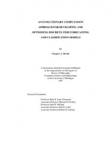
3.6 Nutrient Criteria Below we examine the information that we used and the logic that we followed to define an approach for deriving nutrient criteria for Pensacola Bay. We then apply the approach to derive hypothetical criteria. We also examine how the scientific information about the bay influenced the approach that was followed. In our evaluation of Pensacola Bay water quality, we examined the environmental history of the bay, current attributes of the phytoplankton community, the prevalence of low DO (i.e., hypoxia), the status of seagrass (SAV) habitats, and the status of land use and nutrient exports from the watershed. We related these elements via a conceptual model of key ecosystem processes related to nutrients (Figure 2). We also evaluated water quality in Pensacola Bay in a 22

Our analysis began with the historical data. We concluded that there were no data to indicate clearly that water quality in Pensacola Bay had declined because of nutrients (box A in Figure 10). This effectively eliminated the possibility of deriving criteria based, in large part, on a historical reference condition approach (box F). Had the available historical data shown a substantial decline in water quality, we may have considered a greater role for historical data in deriving nutrient criteria (box F). Even if this had been the case, additional supporting information still would be useful to further evaluate and support the values. Comparison of water quality in Pensacola Bay with other estuaries (box B in Figure 10) in its ecoregion-based class (Table 2, Figure 5) showed that water quality was often among the best in the class, and that it was not degraded relative to the class. Because current values for many water quality indicators were better than the comparison values obtained from the percentile approach, it did not seem reasonable to use these values as criteria. If, on the other hand, the comparison values determined via the percentile approach were better than current values, one might reasonably F A Is water quality begin with the comparison Historical reference values Yes degraded relative to a may inform nutrient criteria values as criteria, then documented pristine development historical condition? provide additional No, or inconclusive supporting evidence as possible (box G). G B Values derived from Is water quality Yes percentile approach may be Despite finding degraded compared useful for criteria to similar estuaries? comparatively good water development quality in terms of nutrient No, or inconclusive concentrations, water clarity, J C Additional and chlorophyll-a, Pensacola D Are uses impaired by monitoring and Are nutrient loads Yes conditions commonly Bay has both significant condition significantly enriched due to associated with nutrient assessment anthropogenic causes? bottom water hypoxia and overenrichment? needed. extensive loss of seagrass habitat, conditions widely Yes No No associated with nutrient E Define criteria based I H Nutrient-response enrichment in estuaries (box on current water Define criteria relationships or related C in Figure 10). Because quality. Identify based on current models needed to set causes of impairment water quality. criteria to resolve degraded hypoxia and seagrass loss if possible. condition. have well-known negative impacts on estuarine Figure 10. Flow diagram illustrating the logical path followed to determine an appropriate approach for determining nutrient criteria for Pensacola Bay (boxes A systems, we expect that through E) and a subset of possible alternative paths (boxes F through J) that may human and aquatic life uses have been followed had the scientific findings been different.

comparative context by applying a modified percentile approach in an ecoregional analysis of water quality (Figure 5, Table 2). We evaluated these data by posing a series of questions for which the answers, as well as the uncertainty associated with them, influenced the logical progression. It can be informative to consider the questions (below) separately, but they also may be considered part of a logic path (Figure 10). • Has water quality declined relative to a documented historical condition? • Is the estuary degraded in comparison to similar estuaries (i.e., estuaries in the same class?) • Are there environmental measures or indicators of conditions widely associated with nutrient overenrichment? • Are nutrient loads significantly enriched because of anthropogenic causes? At the end of the process, we determined that a nutrient criteria for Pensacola Bay reasonably could be defined by the current water quality conditions (Figure 10). Below, we explain the process, as outlined in Figure 10, in greater detail.

23

were no historical baseline data with which current loading data could be compared, our analysis of current nutrient inputs from rivers, land use in the watershed, and atmospheric nitrogen deposition suggested that it was unlikely that nutrient inputs have increased dramatically. Evaluating water quality in the major rivers entering the bay showed that nutrient export from the watershed was similar to pristine or nearly pristine watersheds. This observation was supported by the absence in the watershed of major causes of increased nutrient export (e.g., low population, minimal row-crop agriculture, low atmospheric nitrogen deposition). One could conclude that reasonable management actions probably could not effect significant reductions in nutrient inputs to the bay via the major tributary rivers. Further research could reduce the scientific uncertainty regarding nutrient loads from the more developed portions of the watershed immediately surrounding the bay, which remain poorly quantified. Ultimately, our approach to developing criteria (box E in Figure 10) was the same as if no impaired conditions were identified (box I). In each situation, we suggest that it is scientifically justified to define water quality criteria as the current water quality conditions because there is little justification for alternative, more stringent criteria. Table 6 outlines hypothetical criteria that are based on summer medians, by salinity zone, for the 1996 to 2004 timeframe. We computed criteria for chlorophyll-a, secchi depth, DIN, PO43-, TN, TP, and DO. For concentration-based water quality indicators (e.g., chlorophyll-a), the criteria include a 10% buffer and a suitable averaging period (e.g., 3 years), such that small climate-driven variations surrounding current water quality would not trigger a determination of impairment. Because we concluded that a portion of the bay may be subject to hypoxia even in the absence of anthropogenic nutrient enrichment, DO criteria for bottom water must accommodate this feature of the ecosystem in some way. Our evaluation of oxygen dynamics in the bay indicates that a sensible approach would define hypoxia and limit the acceptable extent in

are limited by these conditions. Moreover, seagrass loss and hypoxia often increase with anthropogenic nutrient inputs. The juxtaposition of seagrass loss and hypoxia with otherwise good water quality presents a relatively complex picture for nutrient criteria in Pensacola Bay. It appears that much of the loss occurred during the 1950s and 1960s in association with industrial nutrient and organic inputs that were eliminated by the early 1970s. Thus, these causes are not present today. The factors that impede recovery, as well as the prospects and best approach for successful restoration could be understood better through additional research. The significant extent of hypoxia in the bay appears to reflect a natural susceptibility of the bay to hypoxia. It is not clear that realistic reductions in nutrients could eliminate hypoxia. Scientific uncertainty surrounding this conclusion also could be reduced through additional research, particularly improved modeling of the coupled physicalchemical dynamics of the ecosystem. Both SAV loss and hypoxia commonly are associated in estuarine and coastal waters with significant phytoplankton blooms, sometimes including harmful algal species. However, phytoplankton production and biomass in Pensacola Bay are relatively modest compared to other systems. High-biomass phytoplankton blooms occur infrequently; harmful algal blooms are not known to develop in Pensacola Bay but, on occasion, have been transported into the bay from the Gulf of Mexico (Tester and Steidinger, 1997). It appears that Pensacola Bay is prone to adverse impacts resulting from nutrient enrichment and already has been impacted in the past by nutrients, but it may not be demonstrating clear symptoms of nutrient enrichment at present. To better evaluate this hypothesis, we examined nutrient inputs to the bay (box D in Figure 10). EPA did not include evaluating nutrient sources as part of a recommended criteria development process for freshwater systems (U.S. EPA 2000a,b). Rather, this step usually is undertaken as part of the total daily maximum load process. However, this analysis was a useful diagnostic step for Pensacola Bay and could prove to be important for criteria development for other estuaries. Although there 24

Table 6. Suggested nutrient and nutrient-related water quality criteria for Pensacola Bay resulting from the weight-of-evidence approach described herein. All values are 3-year moving averages of summer medians. The quantities are based on observed values (Table 2) that have been adjusted to provide 10% allowance (i.e., 10% higher for concentrations, 10% lower for secchi depth). Parameter Criteria Recommendation Chlorophyll-a Summer median concentration 0.8 m (salinity 0-5), >1.1 m (salinity 5-18), that nutrient inputs are >1.8 m (salinity >18) -1 elevated because of DO Bottom waters below a pycnocline must have oxygen >2.0 mg L except for in an area that may average up to 25% of the mean obvious anthropogenic low water surface area of the bay. causes. Here, a coherent -1 Surface waters or unstratified waters: oxygen >4.0 mg L at all picture emerges and -1 times. 24-hour average oxygen >5.0 mg L would be supported by DIN Summer median