AN APPROACH FOR MODELLING PREFERENCES OF MULTIPLE

AN APPROACH FOR MODELLING PREFERENCES OF MULTIPLE DECISION MAKERS Tommi Tervonen 1,2,3 , Jos´e Figueira 2,3 , Risto Lahdelma 1 , and Pekka Salminen 4 1

Department of Information Technology, University of Turku, FIN-20520 Turku, Finland. E-mails: [email protected], [email protected] 2 Faculdade de Economia da Universidade de Coimbra, Av. Dias de Silva 165, 3004-512 Coimbra, Portugal. E-mail: [email protected] 3 INESC–Coimbra, R. Antero de Quental 199, 3000-033 Coimbra, Portugal 4 University of Jyv¨ askyl¨a, School of Business and Economics, P.O. Box 35, FIN-40014 Jyv¨askyl¨a, Finland. E-mail: [email protected] ABSTRACT Modern decision making problems are discrete and multicriteria by nature, and involve several decision makers (DMs). One of the key questions in this type of problems is how the preferences of the DMs can be modelled. Usually the DMs are not sure of their preferences or will not tell them to the analyst, because they are not able to express their preferences directly. In these type of situations the decision support system should allow modelling of ignorance. Stochastic Multicriteria Acceptability Analysis (SMAA) is a family of methods to aid DMs in discrete decision aiding problems. Dempster-Shafer theory of evidence (DST) allows modelling of ignorance by using belief functions. In this paper we show how the preferences of multiple DMs or other stakeholders can be modelled and combined using DST, and how this information can then be encoded as interval constraints for sets of weights in SMAA. Our contribution has a wide range of practical applications. We present a real-world case study of human resource management in the public sector. It consists of evaluating the quality of education in the University of Turku, Finland. 1. INTRODUCTION Multiple Criteria Decision Aiding (MCDA) problems include many practical questions which have been addressed widely in the literature. One of the most difficult questions is how the preferences of Decision Makers (DMs) or other stakeholders should be modelled? Usually they are modelled by determining a weight for each criterion and other preference parameters (thresholds, catogory profiles, ...). Stochastic Multicriteria Acceptability Analysis (SMAA) is a family of decision support methods to aid DMs in discrete decision making problems with multiple DMs or other stakeholders. SMAA is a quite recent MCDA methodology, but it has had a tremendous impact for dealing with complex real-world decision making

situations since 1998 (see e.g. [1, 2]). SMAA methodology is based on inverse weight space analysis, which means exploring the weight space in order to describe the weights that would make each alternative the most preferred one, of that would give a certain rank for a specific alternative. The SMAA methodology allows modelling of preference information in form of probability distributions, but in practice the preference information is given in simplified form, for example, as intervals for weights or ranking of criteria. When there are multiple DMs, the preference information must be aggregated before it can be used in SMAA computations. The aggregation method may have a great impact on the results of the SMAA analysis. It is crucial that the preference information from a large set of DMs can be elicited efficiently and aggregated in a consistent and theoretically sound way. Dempster-Shafer theory of evidence (DST) is a generalization of Bayesian theory of probabilities that allows representation of ignorance in the probability assignments [3]. In DST, it is also possible to combine the probability assignments in a theoretically sound way. Multiple alternative methods have been introduced for combining the probability assignments (see, e.g. [3, 4]). For these reasons, DST is very suitable for modelling and aggregating the preferences of multiple DMs. In this paper we show how the DST can be used to model and aggregate the preferences of multiple DMs, and how the aggregated preference information can be applied in SMAA models. The method has been introduced in [5]. In this paper we present a case study of evaluating the quality of education at the University of Turku in which the method is applied. This paper is organized as follows: We describe the outline of the new methodology in Section 2. The SMAA approach is introduced in Section 3. The Dempster-Shafer theory of evidence is briefly reviewed in Section 4. In Section 5, we present the framework for applying DST for preference modelling in SMAA. Section 6 contains a case study of a real-world problem of course evaluation.

We end this paper with conclusions and avenues for future research in Section 7.

Multiple DMs DM 1, ... , DMk

Elicitation process

2. OUTLINE OF THE IMPROVED SMAA METHODOLOGY

Apply a preference elicitation model to get the preference information for each DM i , i=1,...,k

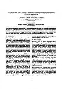
The methodology presented in this paper is for modelling preferences of multiple DMs in SMAA. The preferences of a single DM are modelled by using belief functions as defined by DST. The approach consists of several phases, which we will briefly describe next.

Transform the preference information of each DM into a belief function bpa i , i=1,...,k

Combine the k bpa’s into a single bpa by using the Yager’s rule

Treatment of preference information

1. Transform the preferences of each DM into a belief function (bpa). This can be accomplished, for example, using the method presented in [6].

Compute the belief and plausibility values

2. Combine the belief functions using the Yager’s rule of combination. This results in a single belief function incorporating the preferences of all DMs. 3. Calculate characteristic belief and plausibility values from the combined belief function. 4. Transform the intervals provided by the characteristic values [belief, plausibility] to constraints for sets of weights (the preferences are modelled in SMAA using interval constraints for weights). 5. Apply SMAA, with input consisting of criteria measurements and preference information (interval constraints for weights). The output are certain indicators (confidence factors, acceptability indices, and central weight vectors) characterizing the decision making problem. The complete process is presented in Figure 1. 3. THE SMAA-2 APPROACH The SMAA-2 method [7] has been developed for discrete stochastic MCDA problems with multiple DMs. SMAA-2 applies inverse weight space analysis to describe for each alternative what kind of preferences make it the most preferred one, or place it on any particular position in the ranking. 3.1. Elementary notation The following notation is used in this paper: • {x1 , x2 , . . . , xm } is the set of alternatives. • G = {g1 , g2 , . . . , gn } is the set or family of criteria. • w = (w1 , w2 , . . . , wn ) is a vector of weights. The weights are represented by a weight distribution with joint density function fW (w) in the feasible weight space W . • ξi j are stochastic variables representing imperfect knowledge of criteria measurements. They have a joint density function fX (ξ) in the space X ⊆ Rm×n . Vector ξi = [ξi1 , . . . , ξin ] contains the stochastic criteria measurements of alternative i.

Comprehensive preference elicitation process

Define interval constraints for each subset of weights Set of criteria (finite)

Initial data

Input (preference information) Input

Evaluation matrix

Apply SMAA Outputs

Set of alternatives (finite)

Confidence factors

Acceptability indices

Central weight vectors

Figure 1. The procedure of using DST for preference modelling in SMAA.

• u(xi , w) is the real-valued utility or value function representing the DMs preference structure. The value function maps the different alternatives to real values by using the weight vector w. 3.2. The weight space The weight space can be defined according to needs, but typically, the weights are non-negative and normalized, that is; the weight space is an n − 1 dimensional simplex in n dimensional space: ½ ¾ n n W = w ∈ R : w ≥ 0 and ∑ w j = 1 . (1) j=1

Total lack of preference information is represented in ’Bayesian’ spirit by a uniform weight distribution in W , that is, fW (w) = 1/vol(W ). It should be noticed here, that we use weights in the meaning of scale factors; the weights rescale the value or utility functions in such a way, that the full swing in the scaled function indicates the importance of the criterion (see [8], Sect. 5.4). 3.3. The value function The value function is used to map the stochastic criteria and weight distributions into value distributions u(ξi , w). Based on the value distributions, the rank of each alternative is defined as an integer from the best rank (= 1) to the worst rank (= m) by means of a ranking function m

rank(i, ξ, w) = 1 + ∑ ρ(u(ξk , w) > u(ξi , w)), k=1

(2)

where ρ(true) = 1 and ρ( f alse) = 0. SMAA-2 is then based on analysing the stochastic sets of favourable rank weights Wir (ξ) =

{w ∈ W : rank(i, ξ, w) = r}.

3.4. Descriptive measures provided by SMAA-2 Three types of descriptive measures are obtained as outputs from a SMAA-2 analysis: (1) rank acceptability indices, (2) central weight vectors, and (3) confidence factors. The rank acceptability index (bri ) measures the variety of different preferences that grant alternative xi rank r. It is the share of all feasible weights that make the alternative acceptable for a particular rank, and it is most conveniently expressed percentage-wise. The rank acceptability index bri is computed numerically as a multidimensional integral over the criteria distributions and the favourable rank weights as Z

Z

ξ∈X

fX (ξ)

w∈Wir (ξ)

fW (w) dw dξ.

(4)

fX (ξ) dξ.

(6)

Confidence factors can similarly be calculated for any given weight vectors. The confidence factors measure whether the criteria measurements are accurate enough to discern the efficient alternatives. 3.5. Additional theoretical issues There are several different ways to handle partial preference information in SMAA methods [7]. To our best knowledge, prior to this work there have been no methods, which allow DMs to express ignorance in their preference structures. The DST allows modelling of ignorance, and in this article we will present a novel method for modelling preference information in SMAA by applying DST. Using DST the information is aggregated, and modelled in SMAA as L interval constraints for sums of the subsets of weights. The constraints are given as cmin ` ≤

∑ w j ≤ cmax ` , ∀` = 1, . . . , L,

(7)

where C` is a set of criteria in constraint `. The weight space analysis of SMAA is then performed in the restricted weight space W 0 = {w ∈ W |w satisfies (7)}.

(8)

This means that the uniform weight distribution fW (w) is redefined as ( 1/vol(W 0 ), if w ∈ W 0 , (9) fW (w) = 0, otherwise. Figure 2 illustrates the restricted weight space of a 3criterion problem with a lower and an upper bound for w1 .

Z

Z ξ∈X

ξ∈X:rank(i,ξ,wci )=1

j∈C`

The most acceptable (best) alternatives are those with high acceptabilities for the best ranks. Evidently, the rank acceptability indices are in the range [0,1], where 0 indicates that the alternative will never obtain a given rank and 1 indicates that it will obtain the given rank always with any choice of weights. The first rank acceptability index b1i is called the acceptability index ai . The acceptability index is particularly interesting, because it is nonzero for stochastically efficient alternatives (that is, alternatives that are efficient with some values for the stochastic criteria measurements) and zero for inefficient alternatives. The acceptability index not only identifies the efficient alternatives, but also measures the strength of the efficiency considering simultaneously the uncertainty in criteria measurements and the ignorance in DMs’ preferences. The central weight vector (wci ) is the expected centre of gravity (centroid) of the favourable first rank weights of an alternative. The central weight vector represents the preferences of a “typical” DM supporting this alternative. The central weights of different alternatives can be presented to the DMs in order to help them understand how different weights correspond to different choices with the assumed preference model. The central weight vector wci is computed numerically as a multidimensional integral over the criteria distributions and the favourable first rank weights using wci =

Z

pci =

(3)

Any weight w ∈ Wir (ξ) results in such values for different alternatives, that alternative xi obtains rank r.

bri =

a multidimensional integral over the criteria distributions using

fX (ξ)

w∈Wi1 (ξ)

(pci )

fW (w)w dw dξ/ai .

(5)

The confidence factor is the probability for an alternative to obtain the first rank when the central weight vector is chosen. The confidence factor is computed as

Figure 2. Feasible weight space of a 3-criterion problem with a lower and an upper bound for w1 , 0.2 ≤ w1 ≤ 0.8.

4. THE DEMPSTER-SHAFER THEORY (DST) OF EVIDENCE The DST is an extension of the classical Bayesian theory of probabilities, and it allows modelling of ignorance. But DST can also be used to represent other kind of information than probabilities. For example, in this paper we apply DST to model and to aggregate preference structures.

4.3. The basic probability assignment (bpa) functions DST terminology defines a basic probability assignment (bpa) function as a belief function that assigns probabilities that sum to unity to the propositions and sets of propositions in the frame of discernment. It is defined as m : 2Θ 7→ [0, 1], m(∅) = 0,

4.1. The basis of the theory In the classical Bayesian theory, the probabilities are considered to be objective. This fact stems from the definition of probability: the relative frequency at which an event occurs with. This type of definition does not allow modelling of ignorance, which is important especially when modelling preferences of multiple DMs in the context of MCDA. The DST extends the classical Bayesian theory of probabilities using belief functions. Instead of assigning probabilities to propositions, the belief functions assign probability masses to subsets of the propositions in the frame of discernment (denoted by Θ). The frame of discernment is the set of all propositions.

∑

A⊆Θ

where 2Θ is the powerset of the frame of discernment containing all subsets of Θ (including ∅ and Θ). The bpa’s are also called pieces or bodies of evidence. If there are multiple bpa’s, they can be combined using a combination rule. The Dempster’s rule of combination is [3] m(∅) =0, ∑

m(A) =

• p1 denote the proposition “substance is harmful”, • p2 denote the proposition “substance is not harmful”. Most people do not possess sufficient knowledge required for an informed judgment between the proposition. According to Bayesian theory, in absence of knowledge a probability of 0.5 is assigned to both p1 and p2 . If DST is applied, a probability of 0 is assigned to both p1 and p2 , and 1 to the set Θ representing ignorance. Now suppose we have a third alternative, • p3 denoting the proposition “substance is slightly harmful for humans”. With the modified frame of discernment the Bayesian probabilities would be P(p1 ) = P(p2 ) = P(p3 ) = 0.33, and the DST probabilities P(p1 ) = P(p2 ) = P(p3 ) = 0, P(Θ) = 1. The Bayesian probabilities thus strongly depend on the frame of discernment, and by looking at the example it is evident that DST is more consistent in assignment of the probability masses. Based on the previous example, it should also be noted, that when the Bayesian approach is applied, knowledge and ignorance are indistinguishable. If DST is applied, ignorance can be modelled, and in addition certain metrics can be used for calculating the total amount of ignorance in the belief structure [3].

Ai ∩B j =A

m1 (Ai )m2 (B j ) 1−K

where

4.2. An illustrative example Let us illustrate this by an example. Consider a situation where we have to decide whether a certain chemical substance is harmful to humans. Let:

(10)

m(A) = 1,

K=

∑

(11) , if A 6= ∅,

m1 (Ai )m2 (B j ), and

(12)

Ai ∩B j =∅

m1 and m2 are bpa’s, m is the combined bpa, and A1 , . . . , Ak and B1 , . . . , Bl are their focal elements (subsets), respectively. 4.4. The weight of conflict and the Yager’s rule Let us consider K denoting the weight of conflict, which measures the conflict between two bpa’s. In the Dempster’s rule, the weight of conflict is used for normalizing, meaning that it is distributed among all subsets of propositions. This approach has the downside of distributing the conflict, without any particular reason, to all sets of propositions. In some situations the alternative Yager’s rule of combination may be more suitable [4]: m(∅) =0, m(A) =

∑

m1 (Ai )m2 (B j ), if A 6= ∅, A 6= Θ

Ai ∩B j =A

µ m(Θ) =

∑

¶ m1 (Ai )m2 (B j ) + K.

(13)

Ai ∩B j =Θ

By using Yager’s rule of combination, the weight of conflict is added to the set representing all propositions (the frame of discernment), so the conflict is added to the ignorance represented in the belief structure. We will use Yager’s rule when applying DST for combining preferences in SMAA. 4.5. On the notion of belief and plausibility After all available pieces of evidence have been combined, DST allows characteristic values to be calculated from the bpa’s. The two most important are belief and plausibility. Belief in a set of propositions A measures the probability

mass that is assigned to A or any subset of A. It measures the confidence we have in A, and is defined as Bel(A) =

∑ m(B), for all A ⊆ Θ.

(14)

B⊆A

Plausibility in a set of propositions A measures the probability mass that is assigned to sets that have common elements with A. It is the amount we fail to disbelieve A, and is defined as Pls(A) =

∑

m(B), for all A ⊆ Θ.

(15)

B∩A6=∅

[Bel(A), Pls(A)] is thus the interval for the “true” probability of A when ignorance is taken into account. Ignorance is present not only in basic probability assignments to Θ, but also in those to sets of multiple propositions. For example, assignment of probability 1.0 to a set of propositions {p1 , p2 } means that either of the propositions is certainly true, but there exists no information about which one it is. 5. DST FOR PREFERENCE MODELLING IN SMAA The DST can be used to model preferences of multiple DMs by considering the preferences of each DM as a body of evidence. This means that from the preferences of a DM, we have to form a bpa representing her/his preferences and ignorance. In this bpa, propositions will be the criteria {g1 , . . . , gn }. After this, all bpa’s of different DMs are combined. From the combined bpa we calculate belief and plausibility values for all subsets of weights. The aggregated preferences are then represented as interval constraints [Bel, Pls] for the sums of subsets of weights. Eliciting the preferences and transforming them into bpa’s can be accomplished in multiple ways. The method presented in [6] is applied in the case study of Section 6 to elicit the preferences and to transform them to bpa’s. When applying DST for modelling preferences in SMAA, it may be preferable to apply the Yager’s rule of combination (13), instead of the Dempster’s rule (11). The idea of Yager’s rule is to assume nothing about the nature of conflict. Yager’s rule adds the ignorance to Θ instead of distributing it between all elements. Thus, in presence of conflict, Yager’s rule enlarges all the intervals [Bel, Pls], while Dempster’s rule diminishes them. Because SMAA is designed to perform the analysis using all possible preferences, it is better to apply too wide intervals (and not to assume anything extra) than too narrow ones (and assume that the conflict can be distributed among all subsets). This makes Yager’s rule more suitable in conjunction with SMAA. It must be noticed here, that the following links exist between the notations of DST and MCDA: • p j = g j , meaning that the MCDA criteria are on the role of DST propositions, and • Θ = G, which means that the set of all criteria now replaces the set of all propositions.

6. CASE STUDY: EVALUATING THE QUALITY OF EDUCATION AT THE UNIVERSITY OF TURKU At the Department of Information Technology of the University of Turku, there has been a custom of collecting course feedback since 2001. After each course, students fill a form in which they rate different aspects of the course on a 5-point scale (1–5). Among the aspects rated are, for example, the lecturing skills of the teacher and the quality of the course material. The objective of this study is to analyze a selection of 10 courses taught during the years 2003 and 2004. A grouping of the courses is needed, because we wish to provide recommendations for the staff of the department on how the quality of the education could be improved. The case study applies the method presented earlier in this paper for modelling collective preferences of the students. Also the criteria measurements are based on student evaluations. The courses are thus ranked according to the collective opinions of the “clients”. 6.1. Study data We have chosen to evaluate the following courses: • x1 = Programming I (P1), • x2 = Programming II (P2), • x3 = Data Structures and Algorithms (DA), • x4 = Databases (DB), • x5 = Introduction to Computers (IC), • x6 = Inauguration of Information Systems (IIS), • x7 = Introduction to Computer Science I (ICS1), • x8 = Introduction to Computer Science II (ICS2), • x9 = Modelling of Information Systems II (MIS2), and • x10 = Microprocessors (MP), based on the following criteria: • g1 = Lecturers Level of Expertise (LLE), • g2 = Teaching Skills of Lecturer (LTS), • g3 = Usefulness of Lecture Material (LMU), • g4 = Demonstrators Level of Expertise (DLE), • g5 = Teaching Skills of Demostrator (DTS), and • g6 = Demonstrators Activity in Assuring Comprehension of Exercises (DAC). The course criteria measurements are modelled as Gaussian distributed, with means and standard deviations calculated from the scores given by students in the evaluation forms. The criteria measurements are presented in Table 1.

Course x1 (P1), x2 (P2) x3 (DA) x4 (DB) x5 (IC) x6 (IIS) x7 (ICS1) x8 (ICS2) x9 (MIS2) x10 (MP)

Table 1. Criteria measurements for the case study (mean ± standard deviation). LLE (g1 ) LTS (g2 ) LMU (g3 ) DLE (g4 ) DTS (g5 ) 4.42 ± 0.63 4.08 ± 0.77 3.38 ± 0.92 3.92 ± 0.84 3.44 ± 1.05 4.25 ± 0.68 3.88 ± 0.78 3.68 ± 0.77 4.14 ± 0.59 3.82 ± 0.71 4.37 ± 0.61 4.03 ± 0.75 4.11 ± 0.78 4.32 ± 0.62 4.16 ± 0.63 4.59 ± 0.51 3.65 ± 0.93 3.71 ± 0.99 4.41 ± 0.51 3.94 ± 0.66 4.03 ± 0.84 3.39 ± 0.99 3.74 ± 0.83 4.33 ± 0.53 4.14 ± 0.69 4.41 ± 0.59 3.45 ± 1.06 2.95 ± 1.02 3.77 ± 0.87 3.27 ± 1.08 3.90 ± 0.78 3.04 ± 0.91 3.67 ± 0.90 4.10 ± 0.65 3.78 ± 0.83 3.95 ± 0.60 2.82 ± 0.83 3.69 ± 0.83 4.05 ± 0.53 3.66 ± 0.76 4.26 ± 0.54 3.89 ± 0.63 3.47 ± 0.87 4.00 ± 0.55 3.86 ± 0.68 3.81 ± 0.60 2.86 ± 0.99 3.36 ± 0.95 3.91 ± 0.61 3.48 ± 0.79

6.2. Preference information For eliciting the preference information, a group of 58 students filled a questionnaire rating the criteria used in the study. The questionnaire listed all criteria, and students had to rate them on a 6-point scale (1–6). Half of the questionnaires had the first and last three criteria in inverse order (the 3 criteria concerning lecturer before the criteria concerning demostrator or vice-versa). Using the answers, we defined 58 bpa’s using the method presented in [6]. We combined these bpa’s using the Yager’s rule, which provided as a result a single bpa. This bpa was then used to define lower- and upper bounds for sets of weights as in [5]. The components of the bpa where m(·) ≥ 0.001 with corresponding weight limits are presented in Table 2. The other components with smaller mass assignments are not presented for brevity. Table 2. Components of the bpa of the case study with mass assignment ≥ 0.001. A bpa Bel(A) = wmin Pls(A) = wmax {LLE} 0.072 0.072 0.561 {LTS} 0.211 0.211 0.625 {LMU} 0.024 0.024 0.501 {DLE} 0.034 0.034 0.517 {DTS} 0.028 0.028 0.526 {DAC} 0.052 0.052 0.455 {LLE,DLE} 0.001 0.107 0.675 {LLE,DTS} 0.086 0.186 0.600 {LTS,DLE} 0.013 0.258 0.728 {LMU,DLE} 0.066 0.124 0.550 {LMU,DTS} 0.008 0.061 0.617 {DTS,DAC} 0.001 0.082 0.578 {LLE,LMU,DLE} 0.001 0.199 0.707 G 0.401 1.0 1.0

DAC (g6 ) 3.49 ± 0.97 3.72 ± 0.71 4.07 ± 0.74 3.88 ± 0.78 3.63 ± 0.84 3.27 ± 1.12 3.81 ± 0.84 3.81 ± 0.78 3.59 ± 0.70 3.00 ± 1.00

was done according to the natural scale of the evaluations: minimum score for evaluating a criterion of a course is 1, and the maximum 5. We performed SMAA computations with 100 000 Monte Carlo iterations. The confidence factors and rank acceptability indices are presented percentage-wise in Table 3. The central weight vectors are presented percentage-wise in Table 4. The rank acceptability indices are illustrated graphically in Figure 3. Table 4. Central weight vectors of the case study (in %). The alternatives are in same order as in Table 3. Course LLE LTS LMU DLE DTS DAC DA 19.83 28.41 14.19 13.31 11.50 12.76 DB 20.14 28.36 14.01 13.44 11.38 12.68 P1 20.45 28.68 13.56 13.38 11.27 12.66 P2 20.09 28.49 13.89 13.42 11.40 12.71 IC 19.94 28.18 13.95 13.51 11.68 12.74 IIS 20.51 28.46 13.44 13.48 11.40 12.72 MIS2 19.96 28.55 14.13 13.17 11.59 12.60 ICS1 19.72 27.87 14.15 13.61 11.68 12.97 ICS2 19.59 27.89 14.53 13.27 11.62 13.10 MP 19.51 28.29 14.49 13.62 11.50 12.59

6.3. The SMAA model The SMAA model was constructed with scaling of the value function having 0-point at criterion value 1.0, and 1point at criterion value 5.0. The scaling has a large impact on the results and the shape of the utility function should be accepted by the DMs. In this case study the scaling

Figure 3. The rank acceptability indices of the case study

The strict weight intervals have a visible effect on the acceptability indices: the acceptability indices (b1 ) are al-

Table 3. Rank acceptability indices and confidence factors of the case study (in %), sorted in descending order according to the confidence factors. The highest rank acceptability for each rank appear in boldface and the lowest italized. Course DA DB P1 P2 IC IIS MIS2 ICS1 ICS2 MP

pc 17.8 14.2 12.7 11.1 10.9 9.1 8.1 7.6 4.8 4.1

b1 17.82 14.23 12.72 11.10 10.81 9.18 8.13 7.33 4.55 4.13

b2 15.82 13.21 11.12 11.80 10.24 7.92 10.53 8.10 6.30 4.98

b3 13.94 12.33 10.60 11.96 10.02 7.66 11.92 8.43 7.57 5.57

b4 12.35 11.51 10.12 11.67 9.81 7.86 12.33 8.95 8.61 6.78

most the same as confidence factors (pc ). If the weights are deterministic, the two will be equal. The effect of very imprecise data has an influence on the results: the largest of the confidence factors (for course DA) is only 17.81. The reason for this can be found from the large standard deviations of the criteria measurements. Nevertheless, the results of the SMAA analysis are useful for making conclusions. The imprecision is an inherent attribute of the model, because we are modelling opinions of a large group of heterogenous DMs. When inspecting the results, we should bear in mind, that we have applied a model where ignorance and conflicting opinions are modelled in the last phase (SMAA run) as imprecision. As the preference information was elicited from 58 students, and the criteria measurements modelled based on hundreds of course evaluation forms, we should not expect precise or unanimous results. 6.4. Results Based on the results we divide the courses into three groups, which can be called “good”, “small improvements needed”, and “large improvements needed”. By looking at Table 3, we can distinguish certain courses that obtain high acceptabilities for the best ranks, and low acceptabilities for the worst ranks. DA, DB, P1, and P2 have relatively low acceptabilities for the three worst ranks (b8 − b10 ), and high acceptabilities for the three best ranks (b1 − b3 ). The confidence factors of these courses are also high compared to the other courses. Thus, the first conclusion drawn from the results is, that the majority of the students have an opinion that that these courses are taught well. These courses are placed to the group “good”. The next course in Table 3 (IC) has high acceptabilities for the five best ranks, but it also obtained relatively high acceptabilities for the three worst ranks. This course is separated to the group “small improvements needed”. To this group we place also MIS2, because it obtained relatively low acceptabilities for the best ranks. MIS2 is not placed to the worst group (“large improvements needed”), because it has quite low acceptabilities for the worst two ranks. The remaining courses (IIS, ICS1, ICS2, MP) have

b5 10.65 10.51 10.00 11.23 10.08 8.20 12.45 9.28 9.84 7.78

b6 9.17 9.99 9.71 10.66 9.91 8.76 11.94 10.02 10.93 8.91

b7 7.61 9.07 9.41 9.96 10.14 9.48 11.02 10.59 12.20 10.52

b8 6.06 8.05 9.30 8.96 10.01 10.71 9.51 11.53 13.26 12.63

b9 4.26 6.57 8.95 7.44 9.81 12.63 7.58 12.40 13.86 16.51

b10 2.33 4.54 8.07 5.22 9.17 17.62 4.60 13.37 12.88 22.21

quite high acceptabilities for the worst ranks, and thus we place them in the group “large improvements needed”. ICS2 and MP also have very low confidence factors (under 5%), so even if the acceptability for the best rank would be high, we should not place them into the best group. Table 5 presents the classification of the courses. Table 5. Initial grouping of the courses. Courses DA DB P1 P2 Small improvements needed IC MIS2 Large improvements needed IIS ICS1 ICS2 MP Group Good

The preference information was present in the SMAA model as interval contraints for weights, and the effect of this is evident in the central weight vectors represented in Table 4. Usually (see, e.g. [7]) the central weight vectors have larger deviation. Now most of the central weights are within 1% for all criteria, because the feasible weight space has quite strict contraints. The magnitudes of the central weights for different criteria give insight to the collective preferences; the students seem to value lecturers level of expertise (LLE) and lecturer’s teaching skills (LTS) more than the expertise or the teaching skills of the demonstrator. It might surprise some, that the usefulness of the lecture material is deemed more important than the demostrator’s level of expertise. 6.5. Managerial Implications For making recommendations for the staff of the department we need to identify the shortcomings in the evaluated courses. To do this for the courses in the group “small improvements needed”, we need to find answer to the question: “why are courses IC and MIS2 graded worse than the ones in group “good” by majority of students?”. The

central weight vectors of the alternatives give answer to this question: if the central weight for an alternative is high, then the alternative is performing better with respect to that criteria than to the remaining ones. Because we had strict weight interval constraints present in the model, we have to compare the central weights to the ones of the better alternatives. By looking at the central weights of IC, we can notice that it has a lower central weight for LTS than any course in the class “good”. By looking at the criteria measurements at Table 1, we can see that is has lower mean (3.39) than any of the alternatives in the class “good”. Thus as a recommendation, we think that the lecturer of IC should put more effort on her/his output during the lectures. For MIS2, there is no single central weight which is larger than the others. The criteria measurements of MIS2 are all thus lower than those of the courses in the group “good”. The recommendation for the lecturer of the course MIS2 is thus based on the general preferences: it is most important to improve the level of expertise and the teaching skills. From the central weights of courses ICS1 and ICS2, we can see that they are performing very bad with respect to criteria LTS. The recommendation for the lecturers of those courses is thus to put more effort on the lectures. The low central weight and criteria measurement of LMU for IIS lead us to recommend that the lecturer should improve the lecture material distributed during that course. Also the means of the criteria measurements for the criteria involving demostrator are quite low, so as a second recommendation the demonstrator should improve her/his performance on all areas. The last course, MP, has low criterion measurements for all criteria, and we recommend the lecturer and the demonstrator to think again how the course is taught. By looking at the criteria scores, we can see that LTS and DAC have very low mean values. Thus the first improvements should be that the lecturer improves her/his lecturing skills and the demonstrator spends more time ensuring that all students have understood the solutions of the exercises. 7. CONCLUSIONS AND AVENUES FOR FUTURE RESEARCH In this paper we have presented a method for handling preference information from multiple DMs in SMAA. The method is based on collecting the DMs’ preferences as weights for subsets of criteria, aggregating them using the Yager’s rule of combination and representing them as interval constraints for sums of sets of weights in SMAA. We also presented a case study of university course evaluation in which the method was applied. In the case study we evaluated the quality of education in the Department of Information Technology at the University of Turku, Finland. We used course feedback forms to establish stochastic criteria measurements for the courses, and used questionnaires to elicit preference information from a large group of students. The preference in-

formation was modelled and aggregated using the method introduced in this paper. Based on the results of the analysis, a ranking of the courses could be established, and for the courses with weak performance, improvements could be suggested. This work should not be a “dead-end”. On the contrary, it should be taken further and exploited in other realworld applications. The future theoretical work should address new methods for collecting preferences from the DMs and for transforming them into bpa’s.

Acknowledgements The work of Tommi Tervonen was supported by a grant from Turun Yliopistos¨aa¨ ti¨o. The work of Jos´e Figueira was partially supported by the grant SFRH/BDP/6800/2001 (Fundac¸a˜ o para a Ciˆencia e Tecnologia, Portugal) and MONET research project (POCTI/GES/37707/2001). 8. REFERENCES [1] J. Hokkanen, R. Lahdelma, and P. Salminen, “A multiple criteria decision model for analyzing and choosing among different development patterns for the Helsinki cargo harbor,” Socio-Economic Planning Sciences, vol. 33, pp. 1–23, 1999. [2] R. Lahdelma, P. Salminen, and J. Hokkanen, “Locating a waste treatment facility by using stochastic multicriteria acceptability analysis with ordinal criteria,” European Journal of Operational Research, vol. 142, pp. 345–356, 2002. [3] G. Shafer, A Mathematical Theory of Evidence, Princeton University Press, 1976. [4] R. R. Yager, “On the Dempster-Shafer framework and new combination rules,” Information Sciences, vol. 41, pp. 93–137, 1987. [5] R. Lahdelma, T. Tervonen, J. Figueira, and P. Salminen, “Group preference modelling in SMAA using belief functions,” in Proceedings of the IASTED Conference of Artificial Intelligence and Applications, Innsbruck (to appear), February 2005. [6] T. Tervonen, R. Lahdelma, and P. Salminen, “A method for elicitating and combining group preferences for Stochastic Multicriteria Acceptability Analysis,” Tech. Rep. 638, TUCS - Turku Center for Computer Science, 2004, http://www.tucs.fi. [7] R. Lahdelma and P. Salminen, “SMAA-2: Stochastic multicriteria acceptability analysis for group decision making,” Operations Research, vol. 49, no. 3, pp. 444–454, 2001. [8] V. Belton and T. J. Stewart, Multiple Criteria Decision Analysis - An Integrated Approach, Kluwer Academic Publishers, Dordrecht, 2002.