arXiv:1811.08102v1 [stat.ML] 20 Nov 2018
An interpretable multiple kernel learning approach for the discovery of integrative cancer subtypes Nora K. Speicher 1 and Nico Pfeifer 1,2, 1
∗
Department of Computational Biology and Applied Algorithmics, Max Planck
Institute for Informatics, Saarland Informatics Campus Saarbr¨ ucken, Germany 2
Methods in Medical Informatics,
Department of Computer Science, University of T¨ ubingen, Germany
Abstract: Due to the complexity of cancer, clustering algorithms have been used to disentangle the observed heterogeneity and identify cancer subtypes that can be treated specifically. While kernel based clustering approaches allow the use of more than one input matrix, which is an important factor when considering a multidimensional/manifold disease like cancer, the clustering results remain hard to evaluate and, in many cases, it is unclear which piece of information had which impact on the final result. In this paper, we propose an extension of multiple kernel learning clustering that enables the characterization of each identified patient cluster based on the features that had the highest impact on the result. To this end, we combine feature clustering with multiple kernel dimensionality reduction and introduce FIPPA, a score which measures the feature cluster impact on a patient cluster. Results: We applied the approach to different cancer types described by four different data types with the aim of identifying integrative patient subtypes and understanding which features were most important for their identification. Our results show that our method does not only have state-of-the-art performance according to standard measures (e.g., survival analysis), but, based on the high impact features, it also produces meaningful explanations for the molecular bases of the subtypes. This could provide an important step in the validation of potential cancer subtypes and enable the formulation of new hypotheses concerning individual patient groups. Similar analysis are possible for other disease phenotypes. Availability: Source code for rMKL-LPP with feature clustering and the calculation of fFIPPA scores is available at https://github.molgen.mpg.de/nora/fFIPPA. Contact:
[email protected] ∗ to
whom correspondence should be addressed
1
1
Introduction
Despite the growing amount of multidimensional data available for cancer patients, the optimal treatment for a new patient remains in many cases unknown. In this setting, clustering algorithms are increasingly helpful to identify cancer subtypes, i.e., homogeneous groups of patients that could benefit from the same treatment. Most clustering algorithms, e.g., k-means clustering (Hartigan, 1975) or spectral clustering (von Luxburg, 2007) generate a hard clustering, i.e., each sample is assigned to one cluster, which works well when the clusters are separated. When analyzing cancer data, samples might lie between two or more clusters because they show characteristics of each of them. In these cases, fuzzy or soft clustering methods give additional information, since they assign to each patient a membership probability for each cluster instead of a binary cluster assignment. For the purpose of soft-clustering, fuzzy c-means (Dunn, 1974; Bezdek, 1981) extends the prominent k-means clustering method. To handle the increasing diversity in the data describing the same sample, fuzzy c-means can be combined with multiple kernel learning approaches, either directly as shown by Hsin-Chien Huang et al. (2012) or via application to the result of multiple kernel based dimensionality reduction (Speicher and Pfeifer, 2015). However, after the process of calculating kernel matrices for the input data, the subsequent data integration and the clustering of the samples, interpreting the results is difficult and the crucial features usually remain obscure. This lack of interpretability also hinders the validation of the identified groups in cases where the ground truth is not known. We base our approach on the assumption that sample clusters are not defined by all features but rather by a subset of features which is also the motivation for the technique of biclustering or co-clustering, i.e., the simultaneous clustering of samples and features (Hartigan, 1972). This assumption becomes even more realistic with the increasing number of features within the data types, e.g., for DNA methylation or gene expression data, that are being measured nowadays for a cancer sample. Therefore, our approach combines feature clustering with subsequent data integration and sample clustering, thereby providing several advantages. First, the feature clustering identifies groups of homogeneous features, as typically, even for patients in the same cluster, not all measured features will behave similarly. Consequently, the sample similarities obtained from each of these feature groups are less noisy than the similarities one would obtain based on all the features. Second, due to the learned kernel weights we are able to identify which feature clusters were especially influential for each sample clustering allowing the further characterization of the identified sample clusters. Related work Data integration has been combined with clustering algorithms in different ways. One approach that is regularly used for cancer data is the so-called late integration, where clusterings are combined after they have been retrieved for each data source independently (The Cancer Genome Atlas, 2012). However, signals that might be spread over distinct data types could be 2
too weak in each data source to have an impact on the individual clustering and therefore, might not be present in the final result. To circumvent this problem, different approaches integrate the data at an earlier time point, this way performing intermediate integration. iCluster creates the clustering using a joint latent variable model in which sparsity of the features is imposed by using an l1 norm or a variance-related penalty (Shen et al., 2012). The authors applied their approach to a dataset of 55 glioblastoma patients described by three data types. In a different approach, Wang et al. (2014) extract the sample similarities from each data type and generate sample similarity networks. These can then be fused iteratively by using a message-passing algorithm until convergence to a common integrated network. Another possibility for data integration is multiple kernel learning whose strength lies in its wide applicability in different scenarios, e.g., to integrate data from arbitrary sources or to integrate distinct representations of the same input data. Therefore, it has been combined with a number of unsupervised algorithms in the last years. Yu et al. (2012) developed a multiple kernel version of k-means clustering. The optimization of the weights for the conic sum of kernels is a non-convex problem tackled by a bi-level alternating minimization procedure. A different approach for multiview k-means combines non-linear dimensionality reduction based on multiple kernels with subsequent clustering of the samples in the projection space (Speicher and Pfeifer, 2015). Kumar et al. (2011) extend spectral clustering such that it allows the clustering based on multiple inputs. Here, data integration is achieved by co-regularization of the kernel matrices which enforces the cluster structures in the different matrices to agree. Moving one step further, G¨onen and Margolin (2014) introduced localized kernel k-means, which, instead of optimizing one weight per kernel, uses per-sample weights to have more flexibility to account for sample-specific characteristics. Some of the algorithms described have been applied to cancer data and could show improvements, such as increased robustness to noise in individual data sources and increased flexibility of the model (G¨onen and Margolin, 2014; Speicher and Pfeifer, 2015). However, they do not allow the extraction of importances directly related to specific features or the interpretation of the result on the basis of the applied algorithm, which is especially in unsupervised learning an important step to be able to associate clusters with their specific characteristics. A number of approaches aim at increasing performance and interpretability by incorporating prior knowledge. Multiview biclustering (Le Van et al., 2016) integrates copy number variations with Boolean mutation data, which are transformed into ranked matrices using a known network of molecular interactions between the genes. The subtype identification problem is then formulated as a rank matrix factorization of the ranked data. On breast cancer data, the method could refine the established subtypes which are based on PAM50 classification. Approaches similar to ours concerning the subdivision into feature groups before applying multiple kernel learning were presented by Sinnott and Cai (2018) for supervised survival prediction of cancer patients and by Rahimi and G¨onen 3
(2018) for discriminating early- from late-stage cancers, showing a better interpretability compared to standard approaches. However, in both cases the feature groups are identified using prior knowledge (i.e., gene groups reflecting the memberships to pre-defined biological pathways) and the known outcome of interest is used to train the models, which is not the case for unsupervised clustering.
2
Approach
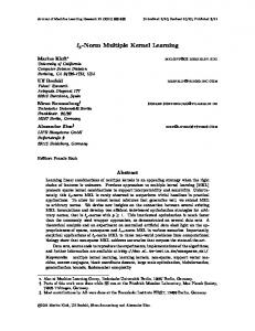
Due to the flexibility of the kernel functions, methods that can handle multiple input kernel matrices allow the integration of very distinct data types, such as numerical, sequence, or graph data, as well as the integration of different preprocessings of the input data. Additionally, the individual up- or downweighting of kernel matrices can account for differences in the quality or relevance of the kernel matrices. However, the features within one data type can be very heterogeneous and might not all be equally important to a meaningful distance measure between the patients. Moreover, for non-linear kernels in general, it is not straightforward how to identify feature importances related to the result. Here, we propose a procedure that combines feature clustering with sample clustering based on multiple kernels, thereby increasing the potential to interpret the result without losing the power of the multiple kernel learning approach. As illustrated in Figure 1, we cluster the features of each data type using k-means such that we can generate one kernel matrix based on each feature cluster. The kernel matrices are then integrated using a multiple kernel learning approach, here regularized multiple kernel learning for locality preserving projection. Based on the low-dimensional projection, we cluster the samples using fuzzy c-means. Our approach provides two advantages compared to standard procedures. First, increasing the homogeneity of the features by identifying feature clusters can reduce the noise in each kernel matrix, this way, a signal that is generated by only a few features can still significantly influence the final result if these features behave very similarly over a subset of samples. Second, the availability of the feature clusters and respective kernel weights allows for increased interpretability of the identified patient clusters as each cluster can be traced back to those groups of features that had the highest influence on the sample similarities. To our knowledge, this is the first extension of a multiple kernel clustering algorithm towards integrative biclustering, where biclustering describes the simultaneous clustering of features and samples, or of rows and columns of a data matrix (Hartigan, 1972).
4
Kernel matrices 1
●●
1
●
0
●
●
●●
● ●
●
−1
● ●
●
●
●
● ● ●
● ● ● ● ● ● ●
−2
● ● ● ● ●
−3
1
●
●
● ● ● ● ●● ● ● ●● ● ● ●●● ● ● ● ● ● ●●
●
−4
● ● ● ● ●
●
● ● ●
2
● ●
●
−2
0
2
4
ID
Cluster 1
Cluster 2
Cluster 3
1 2 3 4
0.02 0.97 0.06 0.18
0.01 0.01 0.02 0.11
0.97 0.02 0.92 0.71
5
0.03
0.96
0.01
6
0.45
0.24
0.31
…
8 41 9 22 36 10 11 1 24 23 2 4 3 39 5 6 7 35 19 20 29 18 25 32 34 40 16 15 14 28 17 12 13 26 27 30 37 38 21 33 31
● ● ● ● ● ●● ● ● ●● ● ● ●●● ● ● ● ● ● ●●
●
−4
4
●
●
−4 0
●
●
●
● ● ● ● ● ● ●
−3
−2
● ●
8 41 9 22 36 10 11 1 24 23 2 4 3 39 5 6 7 35 19 20 29 18 25 32 34 40 16 15 14 28 17 12 13 26 27 30 37 38 21 33 31
11 10 41 4 30 20 40 3 35 5 16 25 2 21 36 27 19 31 22 12 9 14 32 33 29 38 39 24 37 13 7 23 26 6 8 1 15 18 17 34 28
39 33 38 12 30 32 24 19 17 10 22 41 1 6 5 29 9 14 25 16 7 20 28 31 36 27 8 4 21 40 18 15 26 35 3 37 2 23 11 13 34
36 3 20 31 17 37 12 5 19 24 11 10 9 32 21 39 8 34 18 23 35 14 6 7 26 38 29 15 40 13 16 1 22 25 4 2 27 28 33 30
q features
kernel weights
M
● ●
−2
39 33 38 12 30 32 24 19 17 10 22 41 1 6 5 29 9 14 25 16 7 20 28 31 36 27 8 4 21 40 18 15 26 35 3 37 2 23 11 13 34
Ensemble kernel matrix Kernel weights
7 5 18 23 14 35 29 25 38 8 32 24 28 26 9 31 39 22 2 16 1 33 34 6 41 4 19 20 13 11 27 10 36 40 3 30 12 37 21 15 17
Data type II
−1
●
k+1
7 5 18 23 14 35 29 25 38 8 32 24 28 26 9 31 39 22 2 16 1 33 34 6 41 4 19 20 13 11 27 10 36 40 3 30 12 37 21 15 17
●●
●
−4
●
●
●
Sample projection
Optimize
…
●
0
●
24 38 32 14 7 39 8 29 28 34 3 40 11 37 10 41 19 36 27 4 2 22 21 25 33 31 12 30 20 5 6 18 9 35 17 15 1 16 23 26 13
Data type I
k
2
● ● ●● ● ● ●● ● ● ● ● ● ● ● ● ● ●● ● ● ● ● ●● ● ●● ● ● ● ● ●● ● ● ● ●
2
…
24 38 32 14 7 39 8 29 28 34 3 40 11 37 10 41 19 36 27 4 2 22 21 25 33 31 12 30 20 5 6 18 9 35 17 15 1 16 23 26 13
● ● ●● ● ● ●● ● ● ● ● ● ● ● ● ● ●● ● ● ● ● ●● ● ●● ● ● ● ● ●● ● ● ● ●
●●
39 24 7 38 29 30 12 14 9 28 34 32 2 36 22 23 19 5 11 3 10 41 21 4 27 40 8 35 37 20 33 26 17 15 25 16 18 1 31 6 13
p features
36 3 20 31 17 37 12 5 19 24 11 10 9 32 21 39 8 34 18 23 35 14 6 7 26 38 29 15 40 13 16 1 22 25 4 2 27 28 33 30
…
Fuzzy patient clustering
rMKL-LPP
…
11 10 41 4 30 20 40 3 35 5 16 25 2 21 36 27 19 31 22 12 9 14 32 33 29 38 39 24 37 13 7 23 26 6 8 1 15 18 17 34 28
n patients
39 24 7 38 29 30 12 14 9 28 34 32 2 36 22 23 19 5 11 3 10 41 21 4 27 40 8 35 37 20 33 26 17 15 25 16 18 1 31 6 13
…
Feature clustering
projection matrix
Input data
Feature clusterings
Patient clustering
FIPPA: Combined impact scores Patient cluster 1 Patient cluster 2 Patient cluster 3
Data type I Data type II
Figure 1: Overview of the presented approach for two input data matrices. First, feature clustering is performed, here with C = 3. Each feature cluster gives rise to one kernel matrix, which are integrated using rMKL-LPP. This method optimizes one weight for each kernel matrix and a projection matrix, leading to a low-dimensional representation of the samples. Using these learned coordinates, the samples are clustered using fuzzy c-means. Finally, the feature clusters, kernel weights per feature cluster, and the patient clusters are used to calculate FIPPA scores, which describe feature cluster impact on a patient cluster.
3 3.1
Materials and methods Regularized multiple kernel learning for locality preserving projections (rMKL-LPP)
Given a set of M kernel matrices {K1 , ..., KM } that are based on N samples. Multiple kernel learning describes the optimization of a specific weight β for each kernel matrix, such that an ensemble kernel matrix K can be calculated via: M X K= βm KM , with βm ≥ 0. (1) m=1
Regularized multiple kernel learning for locality preserving projections (Speicher and Pfeifer, 2015) optimizes these kernel weights together with a projection matrix such that local neighborhoods are preserved optimally when reducing the dimensionality of the data. The projection matrix A ∈ Rp×N and the 5
kernel weights β ∈ RM are learned via the minimization problem minimize A,β
N X
kAT K(i) β − AT K(j) βk2 wij
(2)
i,j=1
subject to
N X
kAT K(i) βk2 dii = const.
(3)
i=1
with
kβk1 = 1
(4)
βm ≥ 0, m = 1, 2, ..., M.
(5)
KM (1, i) .. N ×M . ∈R .
K(i)
K1 (1, i) .. = .
··· .. . K1 (N, i) · · ·
(6)
KM (N, i)
The projection matrix A consists of p vectors [α1 · · · αp ] that project the data into p dimensions. The weight matrix W and the diagonal matrix D are determined by locality preserving projections using the k-neighborhood Nk (j) of a sample j as follows ( 1, if i ∈ Nk (j) ∨ j ∈ Nk (i) wij = (7) 0, else X and dii = wij . (8) i6=j
The optimization of A and β is performed using coordinate descent. A is optimized by solving a generalized eigenvalue problem, whereas the optimal β is identified using semidefinite programming.
3.2
Fuzzy c-means clustering (FCM)
Given a data matrix X ∈ RN ×l describing N samples xi with l features, FCM identifies C cluster centers vc and assigns the degrees of memberships ui,c for each sample i and cluster c by minimization of the following objective function (Dunn, 1974; Bezdek, 1981): J(U, v) =
N X C X
ufi,c kxi − vc k2
i=1 c=1
subject to
C X
ui,c = 1
∀i
c=1
ui,c ≥ 0 N X
∀i, c
ui,c > 0
i=1
6
∀c.
(9)
The resulting U is an N × C matrix of the degrees of cluster memberships ui,c , which depends on f ≥ 1, a parameter of the method that controls the degree of fuzzification. Choosing f = 1 results in the hard clustering of the samples (i.e., ui,c ∈ {0, 1}); choosing f → ∞ results in uniform cluster probabilities ui,c = 1/C for all i, j.
3.3
Increased interpretability due to simultaneous clustering of features and samples
The impact of each feature cluster m ∈ {1, .., M } on each identified sample cluster c ∈ {1, ..., C} (FIPPAc,m ) can be calculated based on the kernel weights β and the kernel matrices Km using the following equation FIPPAc,m =
1 X βm Km [i, j] , |c|2 x ,x ∈c K[i, j] i
(10)
j
with K being the ensemble kernel matrix. Here, we suppose a hard clustering of the patients, which can either be generated using a hard clustering algorithm or using the modal class of a fuzzy clustering. However, fuzzy clustering provides additional information concerning the reliability of the cluster assignment for each sample. Using these probabilities can make the results more robust given that some samples might have an ambiguous signature and therefore lie between two or more clusters. Given a probability pc (xi ) = p(xi ∈ c) that patient xi belongs to cluster c, the fuzzy FIPPA can be calculated as follows: fFIPPAc,m =
N 1 X βm Km [i, j] . pc (xi )pc (xj ) |N |2 i,j=1 K[i, j]
(11)
The incorporation of the joint probability p(xi ∈ c ∧ xj ∈ c) = pc (xi )pc (xj ) replaces the selection of sample pairs performed in Equation 10 but still allows to downweight the effects of samples that are uncertain or unlikely to belong to c. Moreover, we can separate this overall score into a positive part (fFIPPA+ k,m ) that leads to high intra-cluster similarity and a negative part that leads to high inter-cluster (fFIPPA− k,m ) dissimilarity. For this purpose, we define K+ =
M X
+ βm K m
and
m=1
K− =
M X
− βm K m
(12)
m=1
+ with Km being the positive part of the matrix Km (all negative values set − to zero) and vice versa for Km . For this step, all kernel matrices need to be centered in the feature space, such that the mean of each matrix is equal to zero. When combining Formula 12 with Formula 11, the calculation of the positive
7
and negative fFIPPA is given by fFIPPA+ c,m =
N + 1 X βm K m [i, j] p (x ∧ x ) , c i j 2 + |N | i,j=1 K [i, j]
fFIPPA− c,m =
N − 1 X βm K m [i, j] p (x ⊕ x ) . c i j 2 − |N | i,j=1 K [i, j]
and
(13)
Besides the fact that the two scores are based on the positive and the negative part of the kernel matrices, respectively, the main difference between them is the probability factor for each summand. For the positive fFIPPA, the joint probability pc (xi ∧ xj ) is used to generate high influence for pairs where both partners are likely to belong to cluster c, while for the negative fFIPPA, the exclusive or, defined by pc (xi ⊕ xj ) = (pc (xi ) + pc (xj ) − 2pc (xi )pc (xj )),
(14)
results in an increased factor for pairs of samples of which exactly one has a high probability for c. The fFIPPA scores calculated allow the identification of feature clusters that contribute more than average to the similarity of the samples within a sample cluster and the dissimilarity of the samples in two different clusters, thereby, revealing the underlying basis of the generated clustering.
3.4
Materials
We applied our approach to six different cancer data sets generated by The Cancer Genome Atlas which were downloaded from the UCSC Xena browser (Goldman et al., 2017). The cancer types covered are breast invasive carcinoma (BRCA), lung adenocarcinoma (LUAD), head and neck squamous cell carcinoma (HNSC), lower grade glioma (LGG), thyroid carcinoma (THCA) and prostate adenocarcinoma (PRAD). For each cancer patient, we used DNA methylation, gene expression data, copy number variations, and miRNA expression data for clustering. DNA methylation was mapped from methylation sites to gene promoter and gene body regions using RnBeads (Assenov et al., 2014). Using GeneTrail (St¨ ockel et al., 2016), we mapped the miRNAs to their target genes (i.e., the gene that is regulated by the miRNA) such that the features of each data type were genes. Due to the high number of features available, we performed the whole analysis on the 10% of the features with the highest variance from each data type. For the cluster evaluation, we further leveraged the survival times of the patients for all cancer types except PRAD and THCA. For these two cancer types, survival analysis would not be informative due to the low number of events.
8
4 4.1
Results and discussion Parameter selection
When applying our approach to a data set, we need to choose the number of feature clusters per data type as well as the number of patient clusters. For our experimental validation, we set both parameters to the same value (c ∈ {2, ..., 6}). Feature clustering was performed using k-means before generating the kernel matrices using the Gaussian radial basis kernel function. The parameter of the kernel γ was chosen dependent on the number of features d in the respective feature set based on the rule of thumb γ = 2d12 (G¨artner et al., 2002). We generated three kernels per data type by multiplying this γ with a factor fγ ∈ {0.5, 1, 2} and only used the one kernel matrix providing the highest variance in the first d principal components. The number of neighbors for rMKL-LPP was set to 9 and the the number of dimensions d to 5, as explained in our previous work (Speicher and Pfeifer, 2015). The fuzzification degree f of the soft-clustering algorithm was set to the default value of 2 in concordance with Dunn (1974). If necessary for the subsequent analysis, we assigned each patient to its modal cluster (i.e., the cluster with the highest probability), otherwise, we used the cluster membership probabilities returned by FCM.
4.2
Robustness
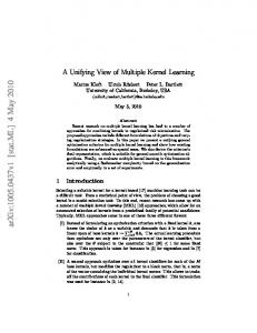
Since each kernel matrix in this approach is constructed on the basis of a feature cluster, slight changes in these initial clusters will propagate through the algorithm and might have an effect on the final result. We repeated the complete approach 50 times with different seeds to analyze the robustness of the final patient clustering. Figure 2 shows the pairwise similarities measured by the Rand index between the final patient clusterings. When including all patients according to their modal class, we observe high reproducibility for all cancer types except LUAD, for which the Rand index is approx. 0.85. When using the class probabilities for each sample to exclude patients where the prediction has a low confidence, here defined as being more than one standard deviation lower than the mean, we observe that the cluster assignments for the remaining patients are more stable for all cancer types including LUAD.
4.3
Survival analysis
To evaluate if a patient clustering could be clinically relevant, we performed survival analysis on the results with C ∈ {2, ..., 6} clusters for each cancer type. To assess the influence of the feature clustering step, we also generated patient clusterings with two established methods: kLPP with the average kernel, and rMKL-LPP without feature clustering, which has been shown to perform well in comparison to other data integration methods (Rappoport and Shamir, 2018). To obtain a fair comparison, the same kernel matrices have been used for all approaches.
9
1.0
●
● ● ● ● ●
● ● ● ● ● ● ● ● ●
●
Rand index
0.95
0.9
0.85
0.8
all samples w/o low confidence samples 0 BRCA
HNSC
LGG
LUAD
PRAD
THCA
Cancer type
Figure 2: Robustness of FC+rMKL-LPP in 50 repetitions. Dark grey boxes indicate Rand indices on the basis of all patients, light grey boxes indicate Rand indices calculated without low confidence samples, i.e., patients with a modal class probability pc more than one standard deviation smaller than the mean of the modal class probabilities. Table 1: For each cancer type and method, we report the most significant results when varying the number of clusters from two to six. Average kLPP stands for kernel locality preserving projection on the (unweighted) average kernel, rMKL-LPP for the standard multiple kernel learning approach with one kernel per data type, and FC + rMKL-LPP represents the proposed approach for which the reported p-values are the median of 50 runs. All three approaches are combined with subsequent fuzzy c-means clustering. C indicates the chosen number of clusters. Cancer average kLPP rMKL-LPP FC + rMKL-LPP p-value C p-value C p-value C BRCA HNSC LGG LUAD
3.7E-2 1.4E-3