An Artificial Immune System Approach with Secondary ... - CiteSeerX

Technical Report IC/2003/65, EPFL, November 2003.

An Artificial Immune System Approach with Secondary Response for Misbehavior Detection in Mobile Ad-Hoc Networks Slaviˇsa Sarafijanovi´c and Jean-Yves Le Boudec

the desire to save battery power: some nodes may run a modified code that pretends to participate in DSR but, for example, does not forward packets. Last, some nodes may also be truly malicious and attempt to bring the network down, as do Internet viruses and worms. An extensive list of such misbehavior is given in [3]. The main operation of DSR is described in Section II-A. In our simulation, we implement faulty nodes that, from time to time, do not forward data or route requests, or do not respond to route requests from their own cache. We consider the problem of detecting nodes that do not correctly execute the DSR protocol. The actions taken after detecting that a node misbehaves range from forbidding to use the node as a relay [1] to excluding the node entirely from any participation in the network [3]. In this paper we focus on the detection of misbehavior and do not discuss the details of actions taken after detection. However, the actions do impact the detection function through the need for a secondary response. Indeed, after a node is disconnected (boycotted) because it was classified as misbehaving, it becomes non-observable. Since the protection system is likely to be adaptive , the ‘punishment” fades out and redemption is allowed [2]. As a result, a misbehaving node is likely to misbehave again, unless it is fixed, for example by a software upgrade. We call primary [resp. secondary ] response the classification of a node that misbehaves for the first [resp. second or more] time; thus we need to provide a secondary response that is much faster than primary response. We chose DSR as a concrete example, because it is one of the protocols being considered for standardization for mobile ad-hoc networks. There are other routing protocols, and there are parts of mobile ad-hoc networks other than routing that need misbehavior detection, for example medium access control protocols. We believe the main elements of our method would also apply there, but a detailed analysis is for further work.

Abstract— In mobile ad-hoc networks, nodes act both as terminals and information relays, and participate in a common routing protocol, such as Dynamic Source Routing (DSR). The network is vulnerable to routing misbehavior, due to faulty or malicious nodes. Misbehavior detection systems aim at removing this vulnerability. In this paper we investigate the use of an Artificial Immune System (AIS) to detect node misbehavior in a mobile ad-hoc network using DSR. The system is inspired by the natural immune system of vertebrates. Our goal is to build a system that, like its natural counterpart, automatically learns and detects new misbehavior. We describe our solution for the classification task of the AIS; it employs negative selection and clonal selection, the algorithms for learning and adaptation used by the natural immune system. We define how we map the natural immune system concepts such as self, antigen and antibody to a mobile ad-hoc network, and give the resulting algorithm for classifying nodes as misbehaving. We implemented the system in the network simulator Glomosim; we present detection results and discuss how the system parameters impact the performance of primary and secondary response. Further steps will extend the design by using an analogy to the innate system, danger signal and memory cells. Index Terms— Mobile, ad-hoc, misbehavior, detection, artificial, immune, clonal selection, learning, adaptive.

I. I NTRODUCTION A. Problem Statement: Detecting Misbehaving Nodes in DSR Mobile ad-hoc networks are self organized networks without any infrastructure other than end user terminals equipped with radios. Communication beyond the transmission range is made possible by having all nodes act both as terminals and information relays. This in turn requires that all nodes participate in a common routing protocol, such as Dynamic Source Routing (DSR) [17]. A problem is that DSR works well only if all nodes execute the protocol correctly, which is difficult to guarantee in an open ad-hoc environment. A possible reason for node misbehavior is faulty software or hardware. In classical (non ad-hoc) networks run by operators, equipment malfunction is known to be an important source of unavailability [18]. In an ad-hoc network, where routing is performed by user provided equipment, we expect the problem to be exacerbated. Another reason for misbehavior stems from

B. Traditional Misbehavior Detection Approaches Traditional approaches to misbehavior detection [1], [3] use the knowledge of anticipated misbehavior patterns and detect them by looking for specific sequences of events. This is very efficient when the targeted misbehavior is known in advance (at system design) and powerful statistical algorithms can be used [4].

The authors are with EPFL, Lausanne, Switzerland. The work presented in this paper was supported (in part) by the National Competence Center in Research on Mobile Information and Communication Systems (NCCRMICS), a center supported by the Swiss National Science Foundation, under the grant number 5005-67322.

1

2

To detect misbehavior in DSR, Buchegger and Le Boudec use a reputation system [3]. Every node calculates the reputation of every other node using its own first hand observations and second hand information obtained from others. The reputation of a node is used to determine whether countermeasures against the node are undertaken or not. A key aspect of the reputation system is how second hand information is used, in order to avoid false accusations [3]. The countermeasures against a misbehaving node are aimed at isolating it, i.e., packets will not be sent over the node and packets sent from the node will be ignored. In this way nodes are stimulated to cooperate in order to get service and maximize their utility, and the network also benefits from the cooperation. Even if not presented by its authors as an artificial immune system, the reputation system in [3], [4] is an example of a (non-bio inspired) immune system. It contains interactions between its healthy elements (well behaving nodes) and detection and exclusion reactions against non-healthy elements (misbehaving nodes). We can compare it to the natural innate immune system (Section II-B), in the sense that it is hardwired in the nodes and changes only with new versions of the protocol. Traditional approaches miss the ability to learn about and adapt to new misbehavior. Every targeted misbehavior has to be imagined in advanced and explicitly addressed in the detection system. This is our motivation for using an artificial immune system approach. C. Artificial Immune System (AIS) Approaches An AIS uses an analogy with the natural Immune System (IS) of vertebrates. As a first approximation, the IS can be described with the “self-nonself” model, as follows (we give more details in Section II-B). Tonsils and adenoids Limph nodes

ISA

ISA

Limph nodes

ISA

Thymus

ISA ISA

Spleen Appendix Bone marrow

Peyer’s patches Limph nodes Limph vesels

ISA

ISA

ISA - (Artificial) Immune System Agent

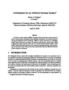
Fig. 1. From the natural IS to an AIS: Making DSR immune to node misbehavior.

The IS is thought to be able to classify cells that are present in the body as self and non-self cells. The IS is made of two distinct sets of components: the innate IS, and the adaptive IS. The innate IS is hard-wired to detect (and destroy) nonself cells that contain, or do not contain, specific patterns on their surface. The adaptive IS is more complex. It produces a large number of randomly created detectors. A “negative selection” mechanism eliminates detectors that match any cell present in a protected environment (bone marrow and the thymus) where only self cells are assumed to be present. Non-eliminated

detectors become “naive” detectors; they die after some time, unless they match something (assumed to be a pathogen), in which case they become memory cells. Further, detectors that do match a pathogen are quickly multiplied (“clonal selection”); this is used to accelerate the response to further attacks. Also, since the clones are not exact replicates, (they are mutated, and mutation rate is an increasing function of affinity between detectors and the pathogen) this provides a more focused response to the pathogen (“affinity maturation”). This also provides adaptation to a changing non-self environment. The self-nonself model is only a very crude approximation of the adaptive IS. Another important aspect is the “danger signal” model [12], [13]. With this model, matching by the innate or adaptive mechanism is not sufficient to cause detection; an additional danger signal is required. The danger signal is for example generated by a cell that dies before being old. The danger signal model better explains how the IS adapts not only to a changing non-self, but also to some changes in self. There are many more aspects to the IS, some of which are not yet fully understood (see Section II-B). D. Artificial Immune Systems - Related Work Hofmeyer and Forrest use an AIS for intrusion detection in wired local area networks [6], [7]. Their work is based on the negative selection part of the self-nonself model and some form of danger signal. TCP connections play the role of self and nonself cells. One connection is represented by a triplet encoding the sender’s destination address, the receiver’s destination address and the receiver’s port number. A detector is a bit sequence of the same length as the triplet. A detector matches a triplet if both have M contiguous equal bits, where M is a fixed system parameter. Candidate detectors are generated randomly; in a learning phase, detectors that match any correct (i.e. self) triplets are eliminated. This is done offline, by presenting only correct TCP connections. Non-eliminated detectors have a finite lifetime and die unless they match a nonself triplet, as in the IS. The danger signal is also used: it is sent by humans as confirmation in case of potential detection. This is a drawback, since human intervention is required to eliminate false positives, but it allows the system to learn changes in the self. With the terminology of statistical pattern classification, this use of the danger signal can be viewed as some form of supervised training. Similarly, Dasgupta and Gonz´alez [21] use an AIS approach to intrusion detection, based on negative selection and genetic algorithms. A major difficulty in building an artificial immune system in our framework is the mapping from biological concepts to computer network elements. Kim and Bentley show that straightforward mappings have computational problems and lead to poor performance, and they introduce a more efficient representation of self and nonself than in [6]. They show the computational weakness of negative selection and add clonal selection to address this problem [9]. In their subsequent papers, they examine clonal selection with negative selection as an operator [10], and dynamical clonal selection [11], showing how different parameters impact detection results. For

3

an overview of AIS, see the book by de Castro and Timmis [20] and the paper by de Castro and von Zuben [19]. In our previous work on building an AIS for misbehavior detection in mobile ad-hoc networks [5] we implemented negative selection. Negative selection is used for learning about the protected system, but it does not provide adaptation to misbehavior. In this work we also implement adaptation, using clonal selection inspired by [10]. Clonal selection provides a faster secondary response to repeated misbehavior, as discussed in Section Section I-A. E. Contribution of this Paper and Organization Our long term goal is to understand whether our previous work, based on the traditional approach [2], can benefit from an AIS approach that introduces learning and adapting mechanisms. In the DSR example, this means adding immune system code to every node, so that it becomes resistant to other nodes’ misbehavior. The first problem to solve is mapping the natural IS concepts to our framework. This is a key issue that strongly influences the detection capabilities. We describe our solution in Section III-B. For the representation of self-nonself and for the matching functions, we start from the general structure proposed by Kim and Bentley [9], which we adapt to our case. Then we define the resulting algorithm, which is based on negative selection, clonal selection and an ad-hoc classification rule. Our main contribution is the definition of a mapping and a construction of an AIS adapted to our case, its implementation in the Glomosim simulator, and its performance analysis. We examine in more detail the effects of clonal selection and show its positive impact on the secondary response time. The rest of the paper is organized as follows. Section II gives background and terminology on DSR and the natural immune system. Section III gives the mapping from the IS to the detection system for DSR misbehavior detection, and the detailed definition of the detection system. Section IV gives simulation specific assumptions and constraints, simulation results and discussion of the results. Section V draws conclusions and describes what we have learned and how we will exploit it in future steps. II. BACKGROUND A. DSR: basic operations DSR is one of the candidate standards for routing in mobile ad hoc networks [17]. A “source route” is a list of nodes that can be used as intermediate relays to reach a destination. It is written in the data packet header at the source; intermediate relays simply look it up to determine the next hop. DSR specifies how sources discover, maintain and use source routes. To discover a source route, a node broadcasts a route request packet. Nodes that receive a route request, add their own address in the source route collecting field of the packet, and then broadcast the packet, except in two cases. The first case is if the same route request was already received by a node; then the node discards the packet. Two received route requests are considered to be the same if they belong to the same route discovery, which is identified by the same

value of source, destination and sequence number fields in the request packets. The second case is if the receiving node is destination of the route discovery, or if it already has a route to the destination in its cache; then the node sends a route reply message that contains a completed source route. If links in the network are bidirectional, the route replies are sent over the reversed collected routes. If links are not bidirectional, the route replies are sent to the initiator of the route discovery as included in a new route request generated by answering nodes. The new route requests will have the destination be the source of the initial route request. The node that initiates an original route request gets usually more route replies, every containing a different route. The replies that arrive earlier than others are expected to indicate better routes, because for a node to send a route reply, it is required to wait first for a time proportional to the number of hops in the route it has as the answer. If a node hears that some neighbor node answers during this waiting time, it supposes that the route it has is worse then the neighbor’s one, and it does not answer. This avoids route reply storms and unnecessary overhead. After the initiator of route discovery gets a first route reply, it sends data over the obtained route. While packets are sent over the route, the route is maintained, in such a way that every node on the route is responsible for the link over which it sends packets. If some link in the route breaks, the node that detects that it cannot send over that link should send error messages to the source. Additionally it should salvage the packets destined to the broken link, i.e., re-route them over alternate partial routes to the destination. The mechanisms just described are the basic operation of DSR. There are also some additional mechanisms, such as gratuitous route replies, caching routes from forwarded or overheard packets and DSR flow state extension [17]. B. The Natural Immune System The main function of the IS is to protect the body against different types of pathogens, such as viruses, bacteria and parasites and to clear it from debris. It consists of a large number of different innate and acquired immune cells, which interact in order to provide detection and elimination of the attackers [14]. We present a short overview based on the selfnonself and the danger models [14], [13]. 1) Functional architecture of the IS: The first line of defense of the body consists of physical barriers: skin and mucous membranes of the digestive, respiratory and reproductive tracts. It prevents the body from being entered easily by pathogens. The innate immune system is the second line of defense. It protects the body against common bacteria, worms and some viruses, and clears it from debris. It also interacts with the adaptive immune system, signaling the presence of damage in self cells and activating the adaptive IS. The adaptive immune system learns about invaders and tunes it’s detection mechanisms to better match previously unknown pathogens. It provides an effective protection against viruses even after they enter the body cells. It adapts to newly encountered viruses and memorizes them for more efficient and fast detection in the future.

4

2) The innate immune system: consists of macrophages cells, complement proteins and natural killer cells. Macrophages are big cells that are attracted by bacteria to engulf the bacteria in the process called “phagocytosis”. Complement proteins can also destroy some common bacteria. Both macrophages and complement proteins send signals to other immune cells when there is an attack. 3) The adaptive immune system: consists of two main types of lymphocyte cells. These are B cells and T cells. Both B and T cells are covered with antibodies. Antibodies are proteins capable of chemically binding to nonself antigens. Antigens are proteins that cover the surface of self and nonself cells. Whether chemical binding takes place between an antibody and an antigen depends on the complementarity of their three-dimensional chemical structures. If it does, the antigen and the antibody are said to be “cognate”. Because this complementarity does not have to be exact, an antibody may have several different cognate antigens. What happens after binding depends on additional control signals exchanged between different IS cells, as we explain next. One B cell is covered by only one type of antibody, but two B cells may have very different antibodies. As there are many B cells (about 1 billion fresh cells are created daily by a healthy human), there is also a large number of different antibodies at the same time. How is this diversity of antibodies created and why do antibodies not match self antigens ? The answer is in the process of creating B cells. B cells are created from stem cells in the bone marrow by rearrangement of genes in immature B cells. Stem cells are generic cells from which all immune cells derive. Rearrangement of genes provides diversity of B cells. Before leaving bone marrow, B cells have to survive negative selection: if the antibodies of a B cell match any self antigen present in the bone marrow during this phase, the cell dies. The cells that survive are likely to be self tolerant. B cells are not fully self tolerant, because not all self antigens are presented in bone marrow. Self tolerance is provided by T cells that are created in the same way as B cells, but in the thymus, the organ behind the breastbone. T cells are self tolerant because almost all self antigens are presented to these cells during negative selection in the thymus. After some antibodies of a B cell match antigens of a pathogen or self cell (we call this event “signal 1b”) that antigens are processed and presented on the surface of the B cell. For this, Major-Histocompatibility-Complex (MHC) molecules are used and their only function. If antibodies of some T cell bind to these antigens and if the T cell is activated (by some additional control signal) the detection is verified and a confirmation signal sent from T cell to B cell (we call this event “signal 2b”). Signal 2b starts the process of producing new B cells, that will be able to match the pathogen better. This process is called clonal selection. If signal 2b is absent, it means that the detected antigens are probably self antigens for which the T cells are tolerant. In this last case, the B cell will die together with its self reactive antibodies. B cells can begin clonal selection without confirmation by signal 2b, but only in the case when matching between B cell antibodies and antigens is very strong. This occurs with a

high probability only for memory B cells, the cells that were verified in the past to match nonself antigens. In the clonal selection phase, a B cell divides into a number of clones with similar but not strictly identical antibodies. Statistically, some clones will match the pathogen that triggered the clonal selection better than the original B cells and some will match it worse. If the pathogens whose antigens triggered clonal selection are still present, they will continue to trigger cloning new B cells that match the pathogen well. The process continues reproducing B cells more and more specific to present pathogens. B cells that are specific enough become memory B cells and do not need co-stimulation by signal 2b. This is a process with positive feedback and it produces a large number of B cells specific to the presented pathogen. Additionally, B cells secrete chemicals that neutralize pathogens. The process stops when pathogens are cleared from the body. Debris produced by the process are cleared by the innate immune system. Memory B cells live long and they are ready to react promptly to the same cognate pathogen in the future. Whereas first time encountered pathogens require a few weeks to be learned and cleared by the IS, the secondary reaction by memory B cells takes usually only a few days. 4) The Danger Signal: is an additional control used for activating T cells. After T cell antibodies bind to antigens presented by MHC of a B cell (signal 1t), the T cell is activated and sends signal 2b to a B cell only if it receives a confirmation signal (signal 2t) from an Antigen Presenting Cell (APC). The APC will give signal 2t to a T cell only if it engulfed the same nonself antigens, which happens only when the APC receive a danger signal from self cells or from the innate immune system. The danger signal is generated when there is some damage to self cells, which is usually due to pathogens. As an example, the danger signal is generated when a cell dies before being old; the cell debris are different when a cell dies of old age or when it is killed by a pathogen. There are many other subtle mechanisms in the IS, and not all of them are fully understood. In particular, time constants of the regulation system (lifetime of B and T cells, probability of reproduction) seem to play an important role in the performance of the IS [15]. We expect that we have to tune similar parameters carefully in an AIS. III. D ESIGN OF O UR D ETECTION S YSTEM A. Overview of Detection System Every DSR node implements an instance of the detection system, and runs it in two phases. In an initial phase, the detection system learns about normal behavior of the nodes with respect to the DSR protocol. During this phase, the node is supposed to be in a protected environment in which all nodes behave well. From received or overheard packets, the node observes the behavior of its neighbors and represent it by the antigens (Section III-C). At the end of this learning phase, the nodes runs the negative selection process and creates its antibodies, which we call detectors (Section III-C). In general terms, the first phase implements a special form of supervised learning, where only positive cases are used for training. After the learning is done, the node may leave the protected environment and enter the second phase where detection and

5

classification are done. In this phase, the node may be exposed to misbehaving nodes. Detectors are used for checking if newly collected antigens represent the behavior of good or bad nodes. If an antigen, created for some neighbor during some time interval, is detected by any of the detectors, the neighbor is considered to be suspicious in that time interval. If there are relatively many suspicious intervals for some node, that node is classified as misbehaving (Section III-D). In the node that did detection, this classification event triggers the clonal selection process (Section III-E). In this process the node adapts its detectors to better detect experienced misbehavior. This results in a better response if the same or similar misbehavior is encountered again. In general terms, the second phase implements a form of re-enforcement learning. The detailed algorithm is given in appendix. B. Mapping of Natural IS Elements to Our Detection System The elements of the natural IS used in our detection system are mapped as follows: • Body: the entire mobile ad-hoc network • Self Cells: well behaving nodes • Nonself Cells: misbehaving nodes • Antigen: Sequence of observed DSR protocol events recognized in sequence of packet headers. Examples of events are “data packet sent”, “data packet received”, “data packet received followed by data packet sent”, “route request packet received followed by route reply sent”. The sequence is mapped to a compact representation as explained in Section III-C. • Antibody: a pattern with the same format as the compact representation of antigen (Section III-C). • Chemical Binding: binding of antibody to antigen is mapped to a “matching function”, as explained in Section III-C. • Bone Marrow: Antibodies are created during an offline learning phase. The bone marrow (protected environment) is mapped to a network with only certified nodes. In a deployed system this would be a testbed with nodes deployed by an operator; in our simulation environment, this is a preliminary simulation phase. C. Antigen, Antibody and Negative Selection 1) Antigens: Antigens could be represented as traces of observed protocol events. However, even in low bit rate networks, this rapidly generates sequences that are very long (for a 100 seconds observation interval, a single sequence may be up to 1 Gbit long), thus causing generation a large number of patterns prohibitive. This was recognized and analyzed by Kim and Bentley in [9] and we follow the conclusions, which we adapt to our case, as we describe now. A node in our system monitors its neighbors and collects one protocol trace per monitored neighbor. A protocol trace consists of a series of data sets, collected on non-overlapping intervals during the activity time of a monitored neighbor. One data set consists of events recorded during one time interval of duration ∆t (∆t = 10s by default), with an additional

constraint to maximum Ns events per a data set (Ns = 40 by default). Data sets are then transformed as follows. First, protocol events are mapped to a finite set of primitives, identified with labels. In the simulation, we use the following list: A= RREQ sent B= RREP sent C= RERR sent D= DATA sent and IP source address is not of monitored node E= RREQ received F= RREP received G= RERR received H= DATA received and IP destination address is not of the monitored node A data set is then represented as a sequence of labels from the alphabet defined above, for example l1 = (EAFBHHEDEBHDHDHHDHD,..) Second, a number of “genes” are defined. A gene is an atomic pattern used for matching. We use the following list: Gene1= #E in sequence Gene2= #(E*(A or B)) in sequence Gene3= #H in sequence Gene4= #(H*D) in sequence where #(’sub-pattern’) is the number of the sub-patterns ’subpattern’ in a sequence, with * representing one arbitrary label or no label at all. For example, #(E*(A or B)) is the number of sub-patterns that are two or three labels long, and that begin with E and end with A or B. The genes are used to map a sequence such as l1 to an intermediate representation that gives the values of the different genes in one data set. For example, l1 is mapped to an antigen that consists of the following four genes:
l2 = 3 2 7 6

Finally, a gene value is encoded on 10 bits as follows. A range of the values of a gene, that are bellow some threshold value, is uniformly divided on 10 intervals. The position of the interval to whom the gene value belongs gives the position of the bit that is set to 1 for the gene in the final representation. The threshold is expected to be reached or exceeded rarely. The values above the threshold are encoded as if they belong to the last interval. Other bits are set to 0. For example, if the threshold value for all the four defined genes is equal to 20, l2 is mapped to the final antigen format: l3 =

0000000010

0000000010

0000001000

0000001000




There is one antigen such as l3 every ∆t seconds, for every monitored node, during the activity time of the monitored node. Every bit in this representation is called a “nucleotide”. 2) Antibody and Matching Function.: Antibodies have the same format as antigens (such as l3 ), except that they may have any number of nucleotides equal to 1 (whereas an antigen has exactly one per gene). An antibody matches an antigen (i.e. they are cognate) if the antibody has a 1 in every position where the antigen has a 1. This is the same as in [10] and is

6

advocated there as a method that allows a detection system to have good coverage of a large set of possible nonself antigens with a relatively small number of antibodies. The genes are defined with the intention to translate raw protocol sequences into more meaningful descriptions. 3) Negative Selection: Antibodies are created randomly, uniformly over the set of possible antibodies. During the offline learning phase, antibodies that match any self antigen are discarded (negative selection). D. Node Detection and Classification Matching an antigen is not enough to decide that the monitored node misbehaves, since we expect, as in any AIS, that false positives occur. Therefore, we make a distinction between detection and classification. We say that a monitored node is detected (or “suspicious”) in one data set (i.e. in one interval of duration ∆t) if the corresponding antigen is matching any antibody. Detection is done per interval of duration ∆t (=10s by default). A monitored node is classified as “misbehaving” if the probability that the node is suspicious, estimated over a sufficiently large number of data sets, is above a threshold. The threshold is computed as follows. Assume we have processed n data sets for this monitored node. Let Mn be the number of data sets (among n) for which this node is detected (i.e. is suspicious). Let θmax be a bound on the probability of false positive detection (detection of well behaving nodes, as if they are misbehaving) that we are willing to accept, i.e. we consider that a node that is detected with a probability ≤ θmax is a correct node (we take by default θmax = 0.06). Let α (=0.0001 by default) be the classification error that we we target. We classify the monitored node as misbehaving if r Mn ξ(α) 1 − θmax √ > θmax (1 + ) (1) n θmax n where ξ(α) is the (1 − α)-quantile of the normal distribution (for example, ξ(0.0001) = 3.72). As long as Equation (1) is not true, the node is classified as well behaving. With default √ . The parameter values, the condition is Mnn > 0.06 + 0.88 ξ(α) n derivation of Equation (1) is given in the appendix. E. Clonal Selection As explained in Section II-B, the antibodies in the IS that are activated by both signal 1b and signal 2b are selected to undergo clonal selection. We define signals 1b and 2b in our setting as follows. Signal 1b. When a misbehaving node is classified as misbehaving (Section III-D), signal 1b is received by the detectors that made the best scores in detecting that node. Signal 2b. We do not implement an exact analog to signal 2b. This is because we do not model helper T-cells (these cells generate signal 2b in the IS) and their activation (Section IIB). Instead, we use a negative selection method, as in [10], defined later in this section, to control the clonal selection process once it starts. Passing the negative selection test by a mutated antibody may be seen as the equivalent of receiving

some type of signal 2b, as it ensures self-tolerance. Indeed, one important function of helper T-cells is providing self-tolerance. The clonal selection mechanism with negative selection works as follows. A fraction W (by default 15%) of the best scored detectors of the node that receive signal 1b enter the clonal selection process, in which each of them will produce one new additional detector. Every detector that enters the process is cloned; the clone is mutated, and if it matches some of the self-antigens in the node’s collection, it is eliminated (negative selection test). This is repeated until one mutated clone is generated that survives the negative selection test. Mutation is defined as random flipping bits of the detector, which occurs with some small probability p (by default 0.1). The newly generated detectors are substituted to the same number of this node’s detectors; the detectors that had the worse score in the detection of misbehaving node that triggered the process are eliminated. For example, let d be a node’s detector that is selected to undergo clonal selection. A possible clonal selection process scenario is as follows. d=

1100010110

1110110010

0010100000

1000001101




From the set (S) of self antigens that the node has collected during the learning phase, let a1 and a2 are two examples: a1 = a2 =

0000000010 0000000010

0000000010 0000000010

0000001000 0000001000


0000000100
0000001000

We see that d does not match a1 or a2 (the matching rule is given in Section III-C.2); it does not match any of the antigens from S, by the rule how it is generated. Let d1 be the first mutated clone of d, which happens to differ from d in 3 bits: d1 =

1100010110

1110110011

0010101000

1000001001




Because d1 matches a2 , d1 is deleted and another mutated clone d2 is created, which happens to differ from d in 4 bits: d2 =

1100010110

1100110010

0011100000

0000011101




We see that d2 does not match a1 or a2 , and assuming that it does not match any other antigen from the set S, d2 becomes a valid detector, and will substitute a badly scored one from the set S. Because the length of the detectors is 40 bits and the mutation probability per bit is 0.1, mutated clones will differ from original detectors from which they are created in 4 bits in average, before negative selection. When detectors are created in learning phase they differ in average in 20 bits before negative selection. This means that clonal selection increases the percentage of the detectors that are similar but slightly different to good scored ones. It is intuitively clear from these facts, and is confirmed by the experiments, that the clonal selection improves the detection results. F. System Parameters In this implementation, the default values of parameters (Table I) are chosen from extensive pilot simulation runs, as a compromise between good detection results and a small memory and computation usage by the detection system.

7

TABLE I D ETECTION S YSTEM PARAMETERS Parameters maximal number of self antigens collected for learning maximal time for collecting self antigens for learning number of detectors number of genes in an antigen number of nucleotides per gene max. number of protocol events recorded in a data set maximal time for collecting a data set (an antigen) accepted misbehavior threshold θmax targeted classification error ratio α percentage of detectors selected for clonal selection probability of mutation per bit

Default values 450 200 s 300 4 10 40 10 s 0.06 0.0001 0.15 0.1

IV. S IMULATION R ESULTS A. Description of Simulation 1) Experimental Setup: We have implemented our detection system in Glomosim [16], a simulation environment for mobile ad-hoc networks. We use the simulator’s DSR code and modify it only to allow nodes’ misbehavior. The detection system code that we add can be run in two versions: with or without clonal selection mechanism. We simulate a network of 40 nodes. The simulation area is a rectangle with the dimensions of 800 m x 600 m. The nodes are initially deployed on a grid with the distance between neighbors equal to 100 m. The mobility model is random waypoint. The speed of nodes is a parameter, and we set it to be constant for one simulation run. The radio range is 380 m. Traffic is generated as constant bit-rate, with packets of length 512 bytes sent every 0.2-1 s. We run two series of experiments: • (Without clonal selection:) In the first set of experiments, clonal selection is disabled. The initial set of detectors generated during the learning phase is used unchanged during the detection and classification phase. • (With clonal selection:) Then we run a second set of experiments, now with clonal selection. Every experiment consists of four consecutive phases, in order to obtain primary and secondary responses. The first phase is learning an initial set of detectors (as in the first experiment). The second phase is detection and classification, but now the detectors start to change and adapt to misbehavior during the phase. This allows us to measure the primary response metrics. In the third phase, nodes do not misbehave, and the system forgets about previous detections, but the set of detectors obtained at the end of the second phase is kept unchanged. The fourth phase is again a detection and classification phase, with the same misbehavior as in the second phase, but the initial set of detectors is now different (it is the set that is achieved at the end of the second phase). This gives the secondary response metrics. The conditions are otherwise the same as in the first set of experiments. We performed 20 independent replications of all experiments, in order to obtain good 90% confidence intervals. For all the simulations, the parameters have the default values (Table I), unless otherwise mentioned.

2) Misbehavior: is implemented by a modifying the DSR implementation in Glomosim. We implemented two types of misbehavior: (1) non-forwarding route requests and nonanswering from its route cache and (2) non-forwarding data packets. A misbehaving node does not misbehave for every packet. In contrast, it does so with fixed probabilities, which are also simulation parameters (default values are 0.6). In our implementation, a node is able to misbehave with different probabilities for the two types of misbehavior. In the simulation we always set both misbehavior probabilities to the same value (what is not necessary). The number of misbehaving nodes is also a simulation parameter (default value is 5). 3) Performance Metrics: We show simulation results with the following metrics: Average Time until Correct Classification: the time until a given node, that is running the detection algorithm, classifies a given misbehaving node as misbehaving for the first time (after a sufficiently large number of positive detections occurred, see Equation (1)), averaged over all pairs hnode i that is running the detection algorithm, node j that is classified as misbehaving by node ii. When we talk about “response time” of the detection system, we refer to this metric. True Positive Classification Ratio: the percentage of misbehaving nodes that are classified as misbehaving. False Positive Classification Ratio: the percentage of well behaving nodes that are mistakenly classified as misbehaving. B. Simulation results 1) Classification capabilities: For all simulation runs, all misbehaving nodes are detected and classified as misbehaving by all their neighbors in the static case and by all nodes in the cases with mobility. The main effect on other classification metrics is by the parameter α, the classification error tolerance (Figure 2). By decreasing the value of α, the false positive classification ratio decreases quickly to very small values, below the value 0.002 (Figure 2(a)), causing a relatively small increase in the time needed for true positive classification (Figure 2(b)). This indicates that it is possible to choose α in the order of 0.0001 and obtain both a very small value of false classification ratio and a small time until classification. 2) Impact of clonal selection: Clonal selection has a significant effect on the secondary response time, which is decreased by a factor 3−4 (Figure 2(b)). The false positive classification ratio is also decreased a little (Figure 2(b)). Another positive effect of clonal selection is a slight decrease in primary response time (Figure 2(b), Figure 3). This slight decrease is more pronounced when the number of misbehaving nodes is large. This is because it is likely that a node that sees a specific misbehaving node for the first time was already exposed to other misbehaving nodes before. If there is only one misbehaving node, this effect does not occur (Figure 3(a)). 3) Effect of other parameters: Figure 3 shows that parameters other than α have a limited effect on the time until classification. The effect of these parameters on the false positive classification ratio is even smaller. The values of obtained false positive classification ratios vary in the very small range between 0.001 and 0.003 (as mainly determined

8

1000 without clonal selection (CS) CS: primary response CS: secondary response

0.016

time until classification [s]

false positive classification ratio

0.02 0.018

0.014 0.012 0.01 0.008 0.006 0.004 0.002

without clonal selection (CS) CS: primary response CS: secondary response

900 800 700 600 500 400 300 200 100

0

0 0.1

0.01

0.001

0.0001

0.00001

0.000001

0.1

0.01

targeted false positive classification

0.001

0.0001

0.00001

0.000001

targeted false positive classification

(a)

(b)

Fig. 2. The AIS main metrics: (a) Average ratio of misclassification for well behaving nodes (false positive) and (b) average time until correct classification for misbehaving nodes versus target false positive classification probability α, for tree cases: without clonal selection (CS), with CS-primary response, with CS-secondary response. Comment: true positive classification ratio is equal to 1, what is not shown on the graphs. 1000

1400

700 600 500 400 300 200

without clonal selection (CS) CS: primary response CS: secondary response

100 0

without clonal selection (CS) CS: primary response CS: secondary response

1200

time until classification [s]

800

time until classification [s]

time until classification [s]

900

1000 800 600 400 200

5

10

15

20

25

30

35

nubmer of misbehaving nodes

(a)

800 700 600 500 400 300 without clonal selection (CS) CS: primary response CS: secondary response

200 100 0

0 0

900

0

0.2

0.4

0.6

misbehavior probability

(b)

0.8

1

0

2

4

6

8

10

12

14

16

speed of nodes [m/s]

(c)

Fig. 3. Behavior of the detection system with parameters change: Time until true positive classification with respect to: (a) number of misbehaving nodes; (b) misbehavior probability; (c) speed of nodes. In all cases target misclassification probability parameter α is set 0.0001. We do not put obtained false positive ratios on the graphs, because they vary in the vary small range between 0.001 and 0.003.

by the value of the parameter α (α = 0.0001)) and this is the reason we do not show them on the graphs. V. C ONCLUSIONS 1) Results obtained so far: We have designed a method to apply an artificial immune system approach for misbehavior detection in a mobile ad-hoc network. Our simulations show good detection capabilities and the effectiveness of clonal selection at providing an accelerated secondary response. As explained in Section I-D, a quick secondary response is of special importance in the case of our protected system. 2) Lessons learned and Future Work: In this early phase, it is premature to draw general purpose conclusions about the performance of the AIS approach. We need more experiments to extend our initial work to more misbehavior and traffic patterns. Instead, we would like to focus now on what the experience of designing this first phase tells us for the future. 3) Mapping IS to AIS: The most difficult problem we encountered was the mapping from the IS to the concrete problem of DSR misbehavior detection. We have followed the approaches in [6], [8] but a large number of fundamental issues remain unclear. At the highest level, we still wonder what is the best choice for a target unit to be detected: the node, or sequence of messages, or a message itself. This choice could have impact on the design challenges and possible use of the detection system. Even if we stay with the mapping we have designed here, questions remain vastly open.

The very definition of genes is one of them. We have defined them in an ad-hoc way, trying to guess the definitions that would have the best detection capabilities. We made sure to have at least two correlated genes per misbehavior, in order to capture it efficiently. Indeed, we propose to use the correlation between genes as an important criterion in selecting the genes defined in the antigen structure. In a next phase, we are planning to automate the process of selecting genes. Correlation between genes from an offered set of genes can be computed from experimental data in a normal operation of the network without misbehaving nodes. Good pairs, triples or k-tuples of genes, which score high crosscorrelation, can be selected automatically. The final selection of candidate genes would still require to be screened by a human expert intervention, but this would be considerably simpler than designing genes from scratch, as we did. One can observe that such a gene selection process is not part of the natural IS, but one can view it as an accelerated selection process. An alternative is to define genes as arbitrary low level bit patterns, and let negative and clonal selection do the job of keeping only the relevant antibodies. This would be more in line with the original motivation for using an AIS. A problem with this approach is that it would require many genes, and the processing effort needed to generate good detectors increases exponentially with the number of genes. A possible angle of attack is based on the observation that the IS is also a resource management system. Indeed, the IS has mechanisms to multiply IS cells and send them to

9

the parts of the body under attack, thus mobilizing resources where and when needed. An analogy here would be to use randomization: in a steady state, only a small, random subset of protocol event sequences is used to create antigens. When an attack is on (signalled by a danger signal, see below), more events are analyzed in the regions that are in danger. In another direction, the response against a specific attack can depend on the intensity of the detection [22]. 4) Innate System and Danger Signal: The model we implemented in this first step could be fortified with the additional mechanisms of the danger signals [13]. i.e. the signal that controls activation of helper T-cells (the danger signal (Section II-B). Danger signals could be defined as network performance indicators (packet loss, delay). In the natural IS, the danger signal is intimately linked to the innate system. Here, the innate system could be mapped to the traditional approach, i.e. a set of pre-defined detection mechanisms as we developed in [4]. It is likely that many new attacks will be accompanied with symptoms that are not new. Thus the innate system could be used as a source of the danger signal as well. This would free resources to focus the adaptive immune system on the detection of truly new, unexpected misbehavior. 5) Regulation: The translation of non-self antigen matching to misbehaviour detection is done in a classical, statistical way. This should be compared to the regulation of B-cell and T-cell clonal division [15], which is algorithmically very different. 6) Parameter Tuning: Even if an appropriate mapping of IS to AIS is found, it remains that the performance is very sensitive to some parameters; the parameters have to be carefully tuned. It is unclear today whether this dependency exists in the IS, and if natural selection takes care of choosing good values, or whether there are inherently stable control mechanisms in the IS that make accurate tuning less important. Understanding this is key to designing not only an AIS as we do here, but also a large class of controlled systems. R EFERENCES [1] Sergio Marti, T.J. Giuli, Kevin Lai, and Mary Baker. Mitigating routing misbehavior in mobile ad hoc networks. In Proceedings of MOBICOM 2000, pages 255–265, 2000. [2] S. Buchegger and J.-Y. Le Boudec. A Robust Reputation System for Mobile ad hoc Networks. Technical Report IC/2003/50, EPFL-DI-ICA, Lausanne, Switzerland, July 2003. [3] S. Buchegger and J.-Y. Le Boudec. Performance Analysis of the CONFIDANT protocol: Cooperation of nodes - Fairness In Distributed AdHoc Networks. In Proceedings of IEEE/ACM Symposium on Mobile Ad-Hoc Networking and Computing (MobiHOC), Lausanne, CH, June 2002. IEEE. [4] S. Buchegger and J.-Y. Le Boudec. The Effect of Rumor Spreading in Reputation Systems for Mobile Ad-hoc Networks. In Proceedings of WiOpt ‘03: Modeling and Optimization in Mobile, Ad Hoc and Wireless Networks”, Sophia-Antipolis, France, March 2003. [5] J. Y. Le Boudec and S. Sarafijanovic. An Artificial Immune System Approach to Misbehavior Detection in Mobile Ad-Hoc Networks. TechReport IC/2003/59, EPFL-DI-ICA, Lausanne, Switzerland, September 2003. [6] S.A. Hofmeyr. An Immunological Model of Distributed Detection and it’s Application to Computer Security. PhD thesis, Department of Computer Sciences, University of New Mexico, April 1999. [7] S. A Hofmeyr and S. Forrest ”Architecture for an Artificial Immune System”. Evolutionary Computation 7(1):45-68. 2000. [8] J. Kim and P.J. Bentley. The Artificial Immune Model for Network Intrusion Detection: 7th European Conference on Intelligent Techniques and Soft Computing (EUFIT’99), Aachen, Germany.

[9] J. Kim and P.J. Bentley. Evaluating Negative Selection in an Artificial Immune System for Network Intrusion Detection: Genetic and Evolutionary Computation Conference 2001 (GECCO-2001), San Francisko, pp. 1330-1337, July 7-11. [10] J. Kim and P.J. Bentley. The Artificial Immune System for Network Intrusion Detection: An Investigation of Clonal Selection with Negative Selection Operator. The Congres on Evolutionary Computation (CEC2001), Seoul, Korea, pp. 1244-1252, May 27-30. [11] J. Kim and P.J. Bentley. Towards an Artificial Immune System for Network Intrusion Detection: An Investigation of Dynamic Clonal Selection. The Congress on Evolutionary Computation (CEC-2002), Honolulu, pp.1015 - 1020, May 12-17, 2002. [12] P. Matzinger. Tolerance, Danger and the Extended Family. Annual Review of Immunology, 12:991-1045, 1994. [13] P. Matzinger. The Danger Model in it’s Historical Contex. Scandinavian Journal of Immunology, 54:4-9, 2001. [14] L.M. Sompayrac. How the Immune System Works, 2nd Edition. Blackwell Publishing, 2003. [15] Tak W. Mak. ‘Order from disorder sprung: recognition and regulation in the immune system. in Phil. Trans. R. Soc. Lond. A (2003) 361, 1235–1250, May 2003. [16] Xiang Zeng, Rajive Bagrodia, and Mario Gerla. Glomosim: A library for parallel simulation of large scale wireless networks. Proceedings of the 12th workshop on Parallel and Distributed Simulations-PDAS’98, May 26-29, in Banff, Alberta, Canada, 1998. [17] D.B. Johnson and D.A. Maltz. The dynamic source routing protocol for mobile ad hoc networks. Internet draft, Mobile Ad Hoc Network (MANET) Working Group, IETF, February 2003. [18] G. Iannaccone C.-N. Chuah, R. Mortier, S. Bhattacharyya, C. Diot. Analysis of Link Failures in an IP Backbone. Proceeding of IMW 2002. ACM Press. Marseille (France). November 2002. [19] De Castro, L. N. and Von Zuben, F. J. (1999), “Artificial Immune Systems: Part I Basic Theory and Applications”, Technical Report RT DCA 01/99. [20] Leandro N. de Castro and Jonathan Timmis, ”Artificial Immune Systems: A New Computational Intelligence Approach” , Springer Verlag, Berlin, 2002. [21] Dipankar Dasgupta and Fabio Gonz´alez, ”An Immunity-Based Technique to Characterize Intrusions in Computer Networks”, IEEE Trans. Evol. Comput., (6)9, June 2002, pp 1081–1088. [22] A. Somayaji and S. Forrest, ”Automated Response Using System-Call Delays.”, Usenix 2000.

A PPENDIX D ETAILED A LGORITHM Here is the detailed detection and classification algorithm that is executed in a node: //learning or detection and classifying phase //may be chosen online; //clonal selection may be enabled or desbled online; //for this an interface to the program exist //through ’phase’ and ’isClonalSelEnabled’ variables // phase=readPhase(); isClonalSelEnabled=readIsCSEnabled(); switch(phase){ case LEARNING{ phaseTimer=maximalLearningTime; numberOfCollectedDataSets=0; collectingDataSetsTimer=0; SetOfDetectors= CreateAnEmptyOrEmptyItIfExistsSetOfDetectors(); numberOfDetectors=0; while(phase==LEARNING){ if(aPacketSentReceivedOrOverheared){ createOrUpdateNeighborsList(); if(collectingDataSetsTimer==0 && numberOfCollectedDataSets