An artificial neural network residual kriging based ...

Advances in Computational Design, Vol. 1, No. 3 (2016) 235-000 235

DOI: http://dx.doi.org/10.12989/acd.2016.1.3.235

An artificial neural network residual kriging based surrogate model for curvilinearly stiffened panel optimization Mohammed R. Sunny2, Sameer B. Mulani3a, Subrata Sanyal4b and Rakesh K. Kapania1c 1

Department of Aerospace and Ocean Engineering, Virginia Polytechnic Institute and State University, Blacksburg, USA 2 Department of Aerospace Engineering, Indian Institute of Technology, Kharagpur 721302, India 3 Department of Aerospace Engineering and Mechanics, The University of Alabama, Tuscaloosa, AL 35487, USA 4 Measurement Science and Engineering Department, Naval Surface Warfare Center (NSWC), Corona Division, P.O. Box 5000, Corona, CA 92878, USA

(Received Janaury 1, 2016, Revised May 26, 2016, Accepted June 7, 2016) Abstract. We have performed a design optimization of a stiffened panel with curvilinear stiffeners using an

artificial neural network (ANN) residual kriging based surrogate modeling approach. The ANN residual kriging based surrogate modeling involves two steps. In the first step, we approximate the objective function using ANN. In the next step we use kriging to model the residue. We optimize the panel in an iterative way. Each iteration involves two steps-shape optimization and size optimization. For both shape and size optimization, we use ANN residual kriging based surrogate model. At each optimization step, we do an initial sampling and fit an ANN residual kriging model for the objective function. Then we keep updating this surrogate model using an adaptive sampling algorithm until the minimum value of the objective function converges. The comparison of the design obtained using our optimization scheme with that obtained using a traditional genetic algorithm (GA) based optimization scheme shows satisfactory agreement. However, with this surrogate model based approach we reach optimum design with less computation effort as compared to the GA based approach which does not use any surrogate model. Keywords: surrogate model; optimization; artificial neural network; kriging; stiffened panel

1. Introduction Design optimization of aerospace systems usually involves high-fidelity analyses and computationally expensive optimization. Surrogate based analysis and optimization (SBAO) is an effective means to tackle this issue. The basic idea of using surrogate models (also called meta Corresponding author, Assistant Professor, E-mail: [email protected] a Assistant Professor, E-mail: [email protected] b Chief Scientist, E-mail: [email protected] c Professor, E-mail: [email protected] Copyright © 2016 Techno-Press, Ltd. http://www.techno-press.com/journals/acd&subpage=7

ISSN: 2383-8477 (Print), 2466-0523 (Online)

Mohammed R. Sunny, Sameer B. Mulani, Subrata Sanyal and Rakesh K. Kapania

models) is to replace the high fidelity, expensive analysis code with a less expensive approximate model. To obtain an accurate approximation, it is necessary to have a good training set and a proper surrogate. Much of the research on surrogates has been done in these two fields, viz., design of experiments and selection and validation of surrogate models. While Queipo et al. (2005), Forrester and Keane (2009), and Jones (2001) have reviewed the state of the art in surrogate model based design optimization in general; Ahmed and Qin (2009) have presented a review of the literature related to its application in the field of aerodynamics. Surrogate models can be broadly classified into two categories-non interpolating and interpolating. Examples of non interpolating (also known as smoothing) surrogate models are polynomial response surface (PRS) and artificial neural networks (ANN). Both of these models are fitted by minimizing the sum of the squared errors at a finite number of selected data points. At the data points, one may not get exact match between the predicted and actual value. Examples of interpolating surrogate models include radial basis neural network (RBNN) and kriging. Response surfaces created by an interpolating surrogate models passes exactly though the data points used for fitting the model. The development of PRS was initiated by Box and Wilson (1951), followed by a comprehensive account of the methods of using PRS by Myers and Montgomery (1995). However, it has been shown to be unsuitable for highly nonlinear and irregular performance problems (Venter et al. 1998, Vavalle and Qin 2007). Several investigations have been carried out to increase the accuracy of the PRS for multi disciplinary optimization (Balabanov et al. 1999), by resizing the design space. To overcome these limitations of PRS, alternative surrogates like kriging and radial basis functions were proposed. Guinta (1997) has shown that quadratic regression polynomial gave better results than kriging. However, Wang et al. (2008) concluded that kriging is superior in nonlinear problems than PRS. An ANN model is a nonparametric regression method. This method utilizes the functional concept of neurons in the brain (Daberkow and Mavris 1998). An ANN is composed of neurons which can be represented as nonlinear transfer functions of the inputs. The main advantages associated with ANN are that: i) it can learn from example and perform the required task, ii) it can create its own organization or representation of the information provided to it, iii) it can retain some of its capabilities even with major network damage. ANN based surrogate models have been successfully used by researchers like Welch et al. (2003), Zaabab et al. (1995) etc. Daberkow and Mavris (1998) critically evaluated the use of ANNs as meta models in aircraft design application, and contrasted this with the RSM method. They found that RSM worked better than ANNs for a problem with few variables and small ranges, but where a large number of variables or extended ranges are involved, ANNs yield a better approximation. Kiranyaz et al. (2009) devised a novel method for automatic generation of ANNs based on a multi dimensional Particle Swarm Optimization. However as ANN is a universal approximator and models the overall nonlinear pattern, in case of the optimization problems where the variation of the objective function with the design variables show very high nonlinearity, an ANN by itself may not be sufficient. Kriging was formally developed by Matheron (Matheron 1963), and was named after a South African mining engineer. Kriging considers the value of a function as a sum of a general trend (could even be a constant) and a systematic departure. Demonstration of the efficiency of kriging for modeling and optimization of deterministic functions can be found in Sacks et al. (1993) and Sacks et al. (1989). Jones and Schonlau (1998) investigated the efficacy of kriging by employing the DACE stochastic model for constructing a global optimization algorithm. Attempts have also been made to increase the performance of kriging by using approaches like Analysis of Variance (ANOVA) (Booker et al. 1998) and gradient data (co-kriging) (Toal and Keane 2011). Kriging,

An artificial neural network residual kriging based surrogate model for…

along with Gaussian functions, is a special type of Radial Basis Function (RBF) method, which uses linear combination of radially symmetric functions to approximate response functions (Keane 2004). RBFs have a special feature that their response decreases (or increases) monotonically with distance from a central point. Michler and Heinrich (2012) have used RBFs to create surrogate models for simulating a fighter aircraft in trimmed state. Demyanov et al. (1998) and Shen et al. (2004) have proposed the use of a hybridized version of ANN and kriging to utilize the benefits of both these models. Demyanov et al. (1998) used the ANN residual kriging model to model climatic data. There are various methods for selecting training points while developing a surrogate model. These include classical methods like fullfactorial design (FFD), partial factorial design (PFD), face-centered cubic (FCC), central composite design (CCD) and D-optimal design. They are easy to implement, but number of points increases rapidly with factors and levels. To counter these difficulties, Space Filling Designs are used. In these designs, points tend to uniformly cover the entire design space. They are used where deterministic errors are expected such as in computer experiments. Latin Hypercube Sampling (LHS) (McKay et al. 1979) and Orthogonal arrays (OA) (Hedayat et al. 1979) employ space filling designs. OA produces uniform design but can generate particular forms of point replication and is sometimes inflexible while LHS does not produce point replicates but is not uniform. To address these concerns, OA-based LHS (Leary et al. 2003, Ye 1998) and other optimal LHS schemes (Palmer and Tsui 2001) have been proposed. The process of selecting a particular surrogate is called validation, in which the generalization error estimates are used to assess the quality of the surrogate and select a model for analysis and optimization. Split sample (SS), Cross Validation (CV) (Myers and Montgomery 1995) and Bootstrapping (Efron 1983) are some of the different schemes that can be used to validate a model. In our optimization problem, we have optimized the shape and size of a stiffened panel with curvilinear stiffeners to minimize its mass keeping its buckling parameter, crippling parameter and von Mises stress parameter within the permissible range. To perform this optimization, we divided the optimization process into two steps. In the first step, we optimize the shape to minimize the buckling parameter. In the second step, we fix the shape and minimize the mass. Variation of the buckling parameter with the design variables is observed to be highly nonlinear. This makes PRS and ANN inefficient for this problem. Following the recommendation of Demyanov et al. (1998), we have used ANN residual kriging for this problem. Among the different sampling methods, we found LHS to be sufficient for application to our problem. However, for higher number of sample points with higher number of design variables, we observed LHS and other sampling methods to be time consuming. So, we designed our own random sampling alogorithm that meet our needs. This work is a part of our research on developing a framework for design optimization of a stiffened plate with curvilinear stiffeners. We call this framework EBF3PanelOpt. In this paper, a brief description of EBF3PanelOpt is given at first. After that, the optimization problem under consideration has been explained. Next, descriptions of ANN, kriging, and ANN residual kriging have been given. After that, our two step optimization process based upon the artificial neural network residual kriging has been explained. We first evaluate the performance of the proposed approach by applying it to optimize the modified Rosenbrock’s function to show the robustness of surrogate model based optimization scheme. Next, we considered two example problems involving mass minimization of a stiffened panel and solved using our proposed artificial neural network residual kriging based surrogate model and traditional GA. Comparison of the two methods has been shown to prove the efficiency of our proposed artificial neural network residual kriging based surrogate model.

Mohammed R. Sunny, Sameer B. Mulani, Subrata Sanyal and Rakesh K. Kapania

2. Motivation  The motivation behind this research came from our need to increase the computational efficiency of the optimization process in EBF3PanelOpt. EBF3PanelOpt developed by the Unitized Structures Research Group at Virginia Polytechninc Institute and State University is a framework for analysis and design of stiffened plates with curvilinear stiffeners. Below is a brief description of the EBF3PanelOpt framework. Msc.Patran (geometry modeling) and Msc.Nastran (finite element analysis) are integrated in the optimization framework, EBF3PanelOpt (Mulani et al. 2010, Mulani et al. 2013, Mulani et al. 2012) using an object oriented script written in Python. EBF3PanelOpt could be coupled with any optimizer to minimize the mass of the curvilinear blade-stiffened panel subjected to constraints on yielding, buckling, and crippling or local failure of the panel. In EBF3PanelOpt, the panel geometry/shape is defined using third-order interpolating B-spline with the help of eight points. The perimeter of panel is defined as one single curve by connecting four edges. The stiffener curve end-points are created by interpolating this perimeter curve. The stiffener curve is represented using third-order uniform rational B-spline using two end-points and a control point, so the stiffener always remains in the panel area. The control-point is defined using interpolation of the panel surface, so the control-point’s x co-ordinate and y co-ordinate have values between 0 and 1. Apart from the definition of stiffener curve points, panel thickness, stiffener thickness, and stiffener height are used as design variables. For two and four blade stiffened panel with uniform panel thickness, the panel has 13 and 25 design variables, respectively. For this work EBF3PanelOpt is utilized along with genetic algorithm (GA) for optimization. It was observed that optimization using GA when performed without any surrogate model requires very high number of evaluation. To address this issue, we developed a surrogate model based optimization scheme that requires less CPU time. 3. Description of the optimization problem The optimization problem is formulated as min f 0 (x) x

f i ( x)  1,

i  1, , m

(1)

A j  x j  B j , j  1, , n.

Here, the design variables xi (i=1,..,m) define the shape, the heights of stiffeners, the thicknesses of the stiffeners, and the thickness of the plate. The objective function f0 is the mass of the plate, constraints fi (i=1,..,3) are the buckling parameter, crippling parameter, and the von Mises stress parameter. Buckling parameter is defined as the reciprocal of the fundamental buckling eigenvalue, von Mises stress parameter is the ratio of the aggregated von Mises stress Kreiselmier-Steinhauster criteria and yield stress. There are total 6Nst+1 design variables, where Nst is the number of stiffeners. Among them, the first 4Nst variables xi (i=1,.., 4Nst) define the shape of the stiffeners, whereas the rest 2Nst+1 variables xi (i=4Nst+1,.., 6Nst+1) define the thickness and height of the stiffeners and the thickness of the plate. To describe the design variables xi, let us take an example of a plate with 2 curvilinear

An artificial neural network residual kriging based surrogate model for…

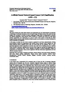
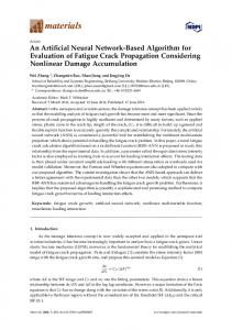
Fig. 1 Top view of a plate with two curvilinear stiffeners

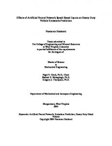
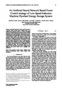
Fig. 2 Front view of a plate with two curvilinear stiffeners

stiffeners. Fig. 1 shows the view of the plate from the top. For this plate we have eight shape variables xi (i=1,..,8) and five size variables xi (i=9,..,13). Variable x4(i-1)+1 and x4i (i=1,2) denote the beginning and end points of the ith stiffener, whereas variables x4(i-1)+2 and x4(i-1)+3 (i=1,2) denote the two control points used to define the shape of the ith stiffener. These variables have values normalized with respect to the perimeter of the plate as shown in Fig. 1. Among the size variables, the first Nst variables xi (i=4Nst+1,.., 5Nst) denote the height of the stiffeners, xi (i=5Nst+1) denote the thickness of the plate and the last Nst variables xi (i=5Nst+2,.., 6Nst+1) denote the thickness of the stiffeners, as described in Fig. 2. Parameters Aj and Bj define the bounds of the design variables. Values of these parameters are Aj=0 (j=1,..,4Nst), Aj=0.01 (j=4Nst+1,.,5Nst), Aj=0.001 (j=5Nst+1,.,6Nst+1), Bj=1 (j=1,..,4Nst), Bj=0.06 (j=4Nst+1,.,5Nst), Bj=0.005 (j=5Nst+1,.,6Nst+1). 4. Artificial neural networks  An ANN is a soft computing system that follows the principle of the operation of biological neurons. It is mostly used for pattern recognition, classification etc. because of its ability to capture and represent complex input/output relationships (Sunny and Kapania 2013, Kim and Kapania

Mohammed R. Sunny, Sameer B. Mulani, Subrata Sanyal and Rakesh K. Kapania

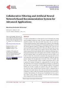
2003). The building blocks of ANN are interconnected processing elements known as the neurons. Like biological neural networks, ANNs acquire knowledge through learning and store knowledge within inter-neuron connection strengths known as synaptic weights. The values of connections (weights) between different neurons are adjusted to enable the neuron to perform a specific task. Figure 3 shows the structure of an ANN with one layer of neurons. The input layer takes the input aj (j=1,..4). Each element of the input layer is connected to the neurons in layer-1. Each connection between an input element aj and the ith neuron is associated with a weight wij. Apart from that, the ith neuron may have a bias bi. Output from the ith neuron is the sum total of weighted inputs and bias operated by an activation function fi. An activation function can be a linear function, the step function, the sigmoid function etc. The output from each neuron can be written as

 m  O  f i   wij p j  bi   j 1 

(2)

A neural network can have a single (or multiple) layers. Depending on the pattern of connections between different layers neural networks can be of two types-feed forward networks and recurrent networks. In the feed forward networks, the data flows from input to the output layers, but there is no feedback connection i.e., there is no flow of data from output to the input layer. Recurrent networks have feedback connections. In some cases, they have dynamic properties i.e., the activations undergo relaxation and evolve to a stable state. The weights and biases of an ANN are adjusted so that a given set of input produces a desired set of output. This is known as the training of an ANN. Training procedures can be divided into two categories-supervised training and unsupervised training. In supervised or associative training, an ANN is provided with a set of input-output pairs. This set of input-output pairs is called the training set. In unsupervised or self organization training, a neural network is trained to respond to a cluster of patterns within the input. Basically, all the training algorithms involving adjustments of weights are variants of the Hebbian learning rule suggested by Hebb in his classic book, Organization of Behavior (Hebb 2002). If the ith neuron in the current layer receives an input xj from the jth neuron in the previous layer and outputs xi, then according to the Hebbian rule, the weight of the connection wij has to be modified by adding Δwij to it, where Δwij is given by the following equation

wij   xi x j γ is called the learning rate. In another rule, difference between the actual and desired activation are used as the objective function to be minimized for adjusting the weights

wij   ( y j  x j ) x j Here, yi is the desired activation. This is called Widrow-Hoff rule or the Delta rule. In a network consisting of single layer of neurons with linear transfer functions, the objective function is a linear function of the weights and biases. So, the derivatives of the objective function with respect to the weights and biases can be easily calculated. In a network with multiple layers of neurons with non linear transfer functions, calculations of the derivatives of the objective function with the weights and biases become complex. Back propagation algorithm of learning makes the calculation of these derivatives easier. Detailed discussions on the different learning rules can be found in Hagan et al. (1996).

An artificial neural network residual kriging based surrogate model for…

Fig. 3 Architecture of an artificial neural network with one hidden layer

5. The kriging model  Kriging is a way of modeling the relationship between the input variables and the output function as a realization of a stochastic process. Detailed description of this method can be found in Jones (2001). The value of the output for an input vector x is modelled as a random process Y( x ) which has a mean µ and variance σ2. The correlation between the random variables at the two points xi and x j is given by the relation

 d  Corr[Yi , Y j ]  exp     l | xil  x jl | pl   l 1 

(3)

Here xil is the lth component of the ith input vector and d is the number of components in each vector. This is just an example of one specific type of correlation function. One can choose from several other types of correlation functions. All these correlation functions should have two properties common - i) when xi = x j , the value of the correlation is 1, and ii) as | xi - x j | tends to infinity, the value of the correlation tends to zero. If we choose the correlation function given by Eq. (3), the parameters θl and pl(l=1,..,d) become the unknown parameters associated with the model. Rest of the modeling process involves the determination of values of the parameters θl, and pl(l=1,..,d) from a training set. The uncertainty about the function’s value at the n training points can be denoted by a vector Y={Y1,..,Yn}T. For this vector, the mean and covariance are µ and cov(Yi, Yj)=σRij. Where Rij is the correlation between Yi and Yj. If the output vector at the nth training point is {y1, ..,yn}T, then the likelihood of the observed data at the training points is given by P

1 (2 )  | R | n/ 2

n

1/ 2

   y  I   ' R 1  y  I    exp   2 2  

(4)

This likelihood is a function of σ and µ, which are function of θl, and pl(l=1,..d). By maximizing P, optimum values of θl, and pl(l=1,..d) are obtained. We denote the optimum values  of θl, and pl(l=1,..d) by θˆl and pˆ l . Using this model, the value of output at any point x is

Mohammed R. Sunny, Sameer B. Mulani, Subrata Sanyal and Rakesh K. Kapania

obtained as

y*  μˆ  r' R 1 ( y  Iμˆ )

(5)

Here, μˆ l is the value of µ obtained using the values of θˆl and dˆl and r’ is a vector where the ith element ri is given by Corr[Yi,Y*]. 6. The artificial neural network residual kriging Modelling using the ANN residual kriging method involves two steps-training an ANN and fitting a kriging model to the data. Let us suppose that we have a training set consisting of n input vectors x1 to xn and n outputs y1 and to yn. In the first step, we train an ANN using this training set. The architecture of the ANN depends on the user’s choice. Using the ANN, we predict the values of the output at the training points using the trained ANN. Let us denote the ANN predicted output at the ith training point as yni. Next, we find out the residue yri=yi-yni at all the data points (i=1,..,n). We define a new training data set that has x1 to xn as the inputs and yr1 to yrn as the outputs. By using this new training data set, we fit a kriging model. This completes the development of an ANN residual kriging  model. Total output at a point x from this model will be the sum of the output obtained from the ANN and the kriging model.

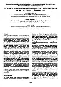
7. The two step optimization process  The surrogate model based optimization was performed in an iterative way. Each iteration involves two steps. In the first step, the size variables are fixed and the buckling parameter is minimized by considering the shape variables as the design variables. In the second step, the shape variables are fixed at the optimum values obtained in the first step and the mass is minimized

Fig. 4 The two step optimization algorithm

An artificial neural network residual kriging based surrogate model for…

keeping the three constraints - buckling parameter, von Mises stress parameter and crippling parameter within the permissible values by considering the size variable as the design variables. Afterwords, we fix the size variable at the optimum values obtained by performing the size optimization at the previous iteration and perform the shape optimization. Again we fix the shape variables at the optimum values and perform the size optimization. The iteration continues until the difference in the values of the optimum mass obtained at two successive iterations is less than a tolerance ɛm defined by the user. Fig. 4 shows the schematic view of this iterative optimization procedure. In the first step, we consider the whole design space for both shape and size optimization. In each successive iteration, we consider a smaller design space around the optima obtained in the previous iteration for both shape and size optimization.

8. The optimization process using the surrogate model based approach 8.1 Sampling algorithm Both the shape and size optimization steps involve random sampling. Before describing each of the shape and size optimization steps it is necessary to describe the sampling algorithm used in those steps. According to our sampling algorithm, the jth element of the ith sample is xsij   Rnd  ( Rshj  1)  / ns

Here, ns is the total number of samples generated. Here Rnd is a random quantity between 0 and 1. Rsh is an array that contains a random combination of the integers ranging from 1 to ns. The jth element of this array is Rshj. 8.2 Modified rosenbrock’s function Before applying our optimization scheme to a complex problem involving shape and size optimization, we evaluated its performance on a standard bench-mark problem, optimization of the modified Rosenbrook’s function. The optimization problems involves the minimization of a modified version of the classical Rosenbrocks’s function (Rossenbrock 1960, Perex et al. 2012) with N dimensional constraint. The optimization problem can be formulated as min x

 n

i 1

100  xi  xi 12   1  xi  2

  0.1   x  1   x n

i 1

3

i

i 1

2



2



 1  0

(6)

-5.12 j  x j  5.12 j , j  1, , N .

Here, N is the number of design variables considered. This optimization was performed in one step i.e., we did not have to break the optimization in different steps unlike the optimization of the stiffened plate described in the next two sub sections. For the surrogate model based optimization, the objective function was modified as shown in Eq. (7) to account for the constraint f mod  f 0  w1 f1 H( f1 )

(7)

Mohammed R. Sunny, Sameer B. Mulani, Subrata Sanyal and Rakesh K. Kapania

Here, f0 is the objective function and f1 is the nonlinear constraint shown in Eq. (6). The function H(f1) has a value zero when f10. At first, we generate a set of n1 sample points using x  [ x1 , x2 ,..., xn ] the random sampling algorithm described in the previous subsection. After that, we evaluate fmod at all the sample points. We define the set y={y1,y2,..,yn1}, where yi is the value of fmod at the ith sample point. Next, we develop an ANN residual kriging model considering the pair of xz and yz as the training set. Now, we find the sample point that has the minimum value of y. Let us denote this value as ymin. Next, we generate N1(N1>>n1) set of new sample points. According to Jones (2001), the probability of fmod having a value (ymin-I) at any of these new sample points x is given by P( I ) 

  y  I  y ( x ) 2 exp   min 2  2s ( x ) 2 s ( x )  1

   

(8)

Here, I is a variable which can have a real positive value. We call it the probability of x having an improvement by a value I over yhmin. By integrating P(I) in the range I≡[0, ∞], we get the expected value of improvement E at x . In this way, we determine E at all of these new sample points and arrange them in descending order. We sort out n2 points having the higher values E and update the sets x and y. We fit an ANN residual kriging model using this updated sets x and y and find out ymin. Again, we generate a new set of N1 sample points and sort out n2 points having the higher values E and update the sets x and y. We continue this iteration unless the difference of ymin at two consecutive iterations is below a tolerance value ɛ. The value of ymin at the last iteration is the minimum values of y. The corresponding value of f0 is the minimum value of the objective function. 8.3 Shape optimization

d hi  [ d hi1 , d hi 2 ]

As mentioned before, for shape optimization at each iteration, we keep the size variables fixed. We denote the range of the ith shape variable as dhi≡[dhi1,dhi2] (i=1,…,Nh), where Nh is the number of shape variables. At the first iterative step dhi1=0, and dhi2=1. At the jth iterative step (j>1), d hi1  xˆ hi  ε hi and d hi 2  xˆhi  εhi . Here xˆ hi is the optimum value of the ith shape variable obtained in the previous iteration, and ɛhi