An Assessment of Data Requirements and Data Transfer ... - CiteSeerX

NISTIR 6216

An Assessment of Data Requirements and Data Transfer Formats for Layered Manufacturing Anne L. Marsan Vinod Kumar Debasish Dutta Michael J. Pratt

U.S. DEPARTMENT OF COMMERCE Technology Administration National Institute of Standards and Technology Manufacturing Engineering Laboratory Manufacturing Systems Integration Division Gaithersburg, MD 20899

NISTIR 6216

An Assessment of Data Requirements and Data Transfer Formats for Layered Manufacturing Anne L. Marsan Vinod Kumar Debasish Dutta Michael J. Pratt

U.S. DEPARTMENT OF COMMERCE William M. Daley, Secretary of Commerce

EN

T OF C O

M

ICA

CE

DEPA

ER

TE

ER

UNI

September 1998

M

M

National Institute of Standards and Technology Raymond G. Kammer, Director

RT

Technology Administration Gary Bachula, Acting Under Secretary for Technology

D

ST

M ATES OF A

Disclaimer Certain commercially available hardware and software products are identified in this report to provide representative examples of current practice and to facilitate understanding of the issues discussed. Their identification does not imply any approval or endorsement of those products by the National Institute of Standards and Technology, nor does it imply that the products identified are necessarily the best available for their purpose. Funding for the preparation of this document was provided by the United States Government. The report is therefore a work of the U.S. Government, and not subject to copyright.

Table of Contents Executive Summary..................................................................................................1 1.0

Introduction..............................................................................................................2 1.1 Description of LM........................................................................................3 1.2 Process planning for LM..............................................................................4 1.3 Data transfer protocol ..................................................................................5

2.0

Process planning for LM..........................................................................................6 2.1 Geometry-related process planning input ....................................................6 2.1.1 Surface models.................................................................................6 2.1.2 Solid models ....................................................................................6 2.1.3 Point data .........................................................................................7 2.1.4 Mathematical data............................................................................7 2.1.5 Image data........................................................................................8 2.1.6 Slice data..........................................................................................8 2.2 Process planning tasks .................................................................................8 2.2.1 Orientation .......................................................................................8 2.2.2 Support structure design ................................................................10 2.2.3 Slicing ............................................................................................12 2.2.4 Path planning .................................................................................15 2.3 Combined design/process planning systems..............................................17 2.4 Summary ....................................................................................................18

3.0

Data transfer protocols for LM ..............................................................................23 3.1 Terminology...............................................................................................23 3.2 The STL format..........................................................................................25 3.2.1 Advantages of the triangulated boundary representation and the STL format.........................................................................25 3.2.2 Disadvantages of the triangulated boundary representation and the STL format.........................................................................26 3.3 Alternatives to STL....................................................................................31 3.3.1 STH - Surface Triangles Hinted format .........................................32 3.3.2 CFL - Cubital Facet List format.....................................................32 3.3.3 RPI (Rensselaer Polytechnic Institute) format...............................32 3.3.4 STEP - Standard for the Exchange of Product Data ......................32 3.3.5 Discussion ......................................................................................34 3.4 Slice Formats for LM.................................................................................34 3.4.1 CLI - Common Layer Interface .....................................................35 3.4.2 LEAF - Layer Exchange ASCII Format ........................................35 3.4.3 HP-GL - Hewlett Packard Graphics Language..............................36 3.4.4 SLC formats ...................................................................................36 3.4.5 STEP ..............................................................................................36 3.4.6 Discussion ......................................................................................36

3.5 3.6

Motivation for alternate 3D representations ..............................................37 Comparison of 3D and slice formats .........................................................38

4.0

Conclusions............................................................................................................42

5.0

Acknowledgments..................................................................................................44

6.0

Addendum - Recent developments ........................................................................45

7.0

Glossary of Acronyms ...........................................................................................46

8.0

References..............................................................................................................48

An Assessment of Data Requirements and Data Transfer Formats for Layered Manufacturing Anne L. Marsan, Vinod Kumar, Debasish Dutta Department of Mechanical Engineering and Applied Mechanics The University of Michigan Ann Arbor, MI 48109-2125 Michael J. Pratt (Guest Researcher, from Rensselaer Polytechnic Institute) National Institute of Standards and Technology Manufacturing Systems Integration Division Building 220, Room A127, Gaithersburg, MD 20899-0001 E-mail: [email protected]

Executive Summary This report surveys the present and future data requirements of layered manufacturing (LM) process planning systems, and the ways in which this data is represented and transferred. Process planning for LM includes determining the optimal build orientation, designing support structures, slicing, path planning, and selecting process parameters. Currently, 3D design data is almost invariably transferred to the LM process planning system using a commercially developed format known as STL. However, there is growing dissatisfaction in the LM community with STL and its underlying representation. Proposed alternative formats are described and their advantages and disadvantages discussed. Data output by LM process planning systems is normally stored in one of several slice formats. These are also described. We propose metrics for the evaluation of the 3D model and 2D slice formats and use them to make comparisons. The study reported in this paper provides guidelines for the development of new representations and formats for use in LM. We conclude by recommending extension of the international standard ISO 10303 to cover the electronic transfer of process planning information for LM.

1

1.0 Introduction Layered manufacturing (LM) is a relatively new class of manufacturing techniques. Introduced in the 1980s as a tool for rapid prototyping, the technology has grown quickly because of its proven ability to save time and money during the product development cycle. Prototypes of a new design can be built in a matter of hours without special tooling or large amounts of dedicated operator time. LM techniques and processes are continually being improved, and this fabrication method is now increasingly used to manufacture part tooling, and in limited cases final products. Products that are to be manufactured by one of the LM techniques generally require the use of specialized software and hardware tools throughout their product development cycle. Product development steps for any method of manufacture include product design, process planning and manufacturing. Typical LM product development steps, and the corresponding tools used to perform them, are shown in Figure 1. We have assumed here that a LM technique is used to manufacture a finished product, but the figure might also represent a subset of a more general product development cycle, whose output is a nonfunctional prototype or a mold for tooling manufacture. Product design for LM may include conceptual and detail design stages, and also analysis. Detail design includes geometric modeling. Each design task may incorporate knowledge about one or more LM processes obtained from a process database or designer experience. LM process planning tasks include determining the optimal build orientation, generating support structures, slicing the part into 2D contours, generating scan paths, and choosing process parameters. Process planning software systems for LM are almost invariably optimized for a particular LM technique and cannot be used with alternate techniques. In addition, the intermediate output of one LM process planning software system is not intelligible to another. Manufacturing involves building the part by one of a variety of LM techniques. There is an increasing number of commercially available LM technologies, and experimental methods are under development by many companies and universities. Some LM techniques require a postprocessing stage to improve the surface finish of the manufactured part, which is then typically used to verify the look-and-feel of a design or to test whether it has some desired behavior. Other forms of post-processing include, for example, curing to remove unsolidified resin in the stereolithography process. However, post-processing activities are specific to particular LM processes. Since they are generally not automated and in most cases involve no electronic information transfer, they will not be further considered here. In this report we focus on the process planning stage within the LM product development cycle. This stage involves several separate tasks. These are described in detail in Section 2, where their informational needs are also analyzed. Many different process planning software systems exist, and in general they are isolated islands working independently of one another. In this report we analyze the feasibility of standardizing the informational needs of LM systems and the representation of their input data in order to define a neutral data transfer format suitable for a variety of LM process planning systems. We discuss these issues in the context of the international standard ISO 10303 for product data exchange, informally known as STEP (STandard for the Exchange of Product model data) [85][101].

2

Tasks

Tools

Product Design

Design software Design database Workstation

Process planning

Process planning software Workstation LM hardware Workstation

Build

Post process

Post processing hardware

Test

Testing hardware

Figure 1. Typical product development steps

1.1 Description of LM Layered manufacturing, also known as solid freeform fabrication (SFF), or rapid prototyping (RP) is an additive manufacturing process in which objects are constructed layer by layer, either by a series of parallel planar layers or concentric cylindrical layers. The basic principle is the same in both cases. In the planar case, thin layers of material approximating the cross-sectional shape of the object are added one by one until the entire part has been built. Many LM processes currently exist, using different types of material and layering methods [1]. Processes have been classified in [2] as: photopolymer solidification, material deposition, powder solidification, laminate-based, and hybrid methods. We add weld-based approaches to this classification. The photopolymer solidification approach involves hardening a liquid resin one layer at a time with a laser or ultraviolet lamp. Processes using this approach are stereolithography and solid ground curing (SGC). Material deposition methods deposit single drops or paths of molten plastic or wax to construct each layer of an object. Fused deposition modeling (FDM) is an example of this approach. In powder solidification methods, powdered materials are solidified by adding a binder or sintering with a laser. Parts can be built from ceramics, nylon, polycarbonate, wax or metal composites. Selective laser sintering (SLS) and three-dimensional printing (3DP) are typical powder solidification processes. In laminate approaches the layers are cut with a laser from sheets of paper, cardboard, foil, or plastic and bonded to each other in a stack. The best known example of this approach is laminated object manufacturing (LOM). Weld-based approaches use

3

welding and cladding techniques to build parts out of metals. No commercial systems of this type were available as this report was being written, but research systems, such as the direct metal deposition (DMD) system at the University of Michigan [3], are under development. Hybrid approaches combine one or more of the above mentioned approaches with traditional manufacturing methods. An example of this is shape deposition modeling (SDM), in which molten metal, plastic, or wax is deposited in a thin layer and machined to give a more accurate surface. LM processes were initially used for rapid prototyping to help the designer verify part geometry. They are now increasingly used to manufacture molds for castings. With the introduction of processes that build parts out of metals, LM has very significant potential as a method for final manufacture of one-off and small batch production parts. LM processes have the advantage that they can be used to build very complex geometries (i.e., objects with internal voids, multiple branches, overhangs, and parts contained completely within other parts), without any special tooling. They also allow the manufacture of complete mechanical assemblies in a single operation. However, because LM objects are built layer by layer, their surfaces often have a staircase appearance. LM-produced parts may also have inferior material properties, especially in the build direction, when compared with objects manufactured by other means. Poor surface quality can be overcome either by building a part in thinner slices or by performing finishing operations such as grinding and polishing after it is built. Improved material properties are more difficult to achieve, though newer LM processes are in general aimed at producing stronger parts than older processes. An important proposed application of LM is the manufacture of heterogeneous objects. These may be composed of more than one material, have varying microstructure, have varying material properties throughout, or contain embedded devices. Because material is added incrementally to the object, we are potentially able to access and control the material properties, composition, and microstructure throughout its volume. In addition, we can build the part around embedded devices. This potential fine control of material properties cannot be achieved by most other manufacturing processes because they do not provide access to the interior of the object during manufacture. Emerging design techniques such as the homogenization method for structural topology design [4][5] specify varying material properties throughout the designed object. LM potentially provides the means for producing such artifacts.

1.2 Process planning for LM In all LM processes, a tool is used to add material to the part. In general, the tool moves while the workpiece is held fixed, and details of its motion are controlled according to certain machine settings. Thus in order to drive a LM apparatus, we need tool paths and process parameter settings. For example, the nozzle through which material is extruded in the FDM process is attached to a liquefier head. The head moves so that the nozzle deposits the material along a particular path, which must be calculated in advance for each layer to be laid down. Several machine parameters must be set, such as the speed of the head, the material flow rate, and the acceleration and deceleration of the head when starting, stopping and changing direction. Process parameters may be varied within a layer, and from layer to layer. Process planning is performed to generate the tool paths and process parameters for an object that is to be built by a particular LM process. The steps required are: part orientation, support structure design, slicing the part into 2D contours, path planning, and process parameter selection. The orientation of a part as it is built will affect the time needed to build the part, its material properties, surface quality and need for support structures. Thus before the part is sliced, an orienta-

4

tion must be determined that is optimal when judged by criteria important to the designer. With certain LM processes, layers that form overhangs or enclose voids must have a sacrificial support structure beneath them to support material as it is added. Such supports are built together with the part, then later detached and discarded. Some process planning systems design the supports after the part has been sliced, while others reverse this order. Finally, tool paths are generated and process parameters are set. Typical LM process planning tasks are shown in Figure 2. A more detailed analysis of LM process planning tasks and their informational needs is given in Section 2.

Orientation

Support structure design

Slicing

Path planning

Figure 2. General chain of events for LM process planning

1.3 Data transfer protocol The designer and manufacturer of a LM object will usually be different people, possibly working in separate organizations. It must therefore be possible to transfer design data to the manufacturer so that process planning can be performed and the part can be built. Hence, there is a need for a data transfer protocol to ensure that data is transferred easily and efficiently, without loss or ambiguity. Since a single organization may manufacture parts using several different LM technologies, a unified data transfer protocol is desirable for the entire class of LM processes. Currently, data describing the boundary of an object is most commonly transferred to the process planning system in the form of an STL file. The STL format, discussed in detail later, was originally developed for use with a particular process, stereolithography, but is now widely used by all LM processes. Its name is not an acronym but a file type extension. STL represents the boundary of the object to be manufactured by a mesh of triangular facets. In Section 3.0 we discuss the drawbacks of this representation and its associated STL format and compare it to other formats, some of which supplement the object’s boundary description with other relevant data. Included in that discussion is a brief introduction to STEP (ISO 10303), an international standard currently under development to provide system-independent product data exchange for a wide variety of product classes and life cycle tasks [85][101]. Our comparison of the various data transfer protocols proposed for LM leads to the recommendation in Section 4 that a STEP Application Protocol should be developed for LM process planning. 5

2.0 Process planning for LM This section is primarily concerned with available techniques for performing those LM process planning tasks that require knowledge of the shape of the part, i.e., part orientation, support structure design, slicing and path planning. The other tasks, including process parameter selection and control, require information about the particular LM technique to be used and the desired material properties of the manufactured part. Much experimental work has been done to determine the effects of varying process parameters on such characteristics as strength and dimensional stability of the final part. However, at the time of writing few models of the experimental data have been developed and incorporated into process planning software. Machine settings are usually fixed for specific build scenarios, and the user is given little control over them. This situation may well change as the technology develops further and these aspects of LM become better understood. This is an area of very active research, but it is likely to be some years before the technology becomes sufficiently stable for standardization of the data for anything more than the most basic aspects of process characterization. Accordingly, this topic will not be further discussed in the present document.

2.1 Geometry-related process planning input The most basic data needed by a LM process planning system is a description of the boundary of the object to be manufactured. Additionally, tolerance information, surface finish, material data, process data, etc., should ideally be used in performing certain process planning tasks, as mentioned above. However, since most LM process planning systems currently accept only shape information, we focus on this area. Several types of shape representation exist, and they are briefly described below. They have all been proposed or used (in some cases experimentally) as input to LM process planning systems [1][6]. 2.1.1 Surface models A surface model is generally composed of bounded regions of various kinds of surfaces linked together to form a larger composite surface. The surface types used may include planar and other simple surfaces, and also free-form surfaces such as NURBS (non-uniform rational B-splines). Topological (connectivity) information is not usually present in a surface model, and it is the responsibility of the designer to ensure that the surface regions actually connect along common edges. If this is not carefully done, the model may contain gaps [7]. Surface models may be either closed (enclosing a volume) or open. The validation of closure, like that of connectivity in general, is the designer’s responsibility. Surface models are often used in die design, and frequently exhibit gaps in practice. A specialized type of surface model uses only planar surfaces, and in this case the composite surface is represented by a mesh of planar polygonal facets. If all the facets are triangular, the model can be written out in what is known as the STL format, the most commonly used input format for LM process planning systems. 2.1.2 Solid models As their name implies, solid models are models of volumetric objects. The primary forms of

6

representation available for them are boundary representation (Brep), constructive solid geometry (CSG) and spatial enumeration. Computer-aided design (CAD) systems usually generate Brep models. These are similar to the surface models described above, but there are three important differences. First, the boundary encloses a solid object, and is therefore itself closed. Second, topological or connectivity information is present, specifying how the various surface regions composing the boundary are connected together. Third, and perhaps most importantly, solid modeling systems are designed to provide automatic validation of shape models with regard to geometrical and topological integrity, closure of model interior, etc. [8]. Hence, solid models are in principle well suited for any kind of post-processing. Like a surface model, a solid model may have curved surfaces or it may be composed of planar facets. Besides representing the boundary of an object, a solid model may also have associated attributes describing its interior, such as its density or other material properties. In addition, certain parts of the boundary of the model may be grouped together to form features. This extra information may be used by process planning software to perform its task more efficiently. A triangulated boundary representation can easily be generated from any form of solid model by approximating the surface regions of the object’s boundary with assemblies of planar triangular facets. The process used is the same triangulation algorithm used frequently for mesh generation in finite element analysis. In this process, the chord-height deviation between the actual object surface and the triangular facets can be controlled. This value defines the maximum absolute deviation of any point on the faceted model from the true surface [9]. Alternatively, the maximum relative deviation of a point on any triangle may be specified with respect to the triangle edge length. A triangulated boundary model is a special case of a polyhedral model in which all polygonal facets are triangles. In a general polyhedral model the number of possibilities for degeneracy (as defined later in Section 3.2.2) grows strongly with increasing number of polygon sides per facet. Controlling the accuracy of the approximation then becomes much more difficult. There is the additional problem of ensuring planarity of the polygons, which requires that all vertices of any polygon must be coplanar. This is automatically achieved in the case of boundary triangulation. Thus, approximation algorithms for creating general polyhedra are more complex than those creating triangulated boundaries, and are not as fast, efficient and robust. As mentioned earlier, a triangulated boundary representation can be written out in the STL format and used as input to an LM process planning system. Some systems, however, will accept a general Brep or CSG solid model representation as input. 2.1.3 Point data This form of input may be used when an existing part is to be duplicated. The part is reverse engineered by scanning it with a 3D shape digitizer. Coordinate measuring machines (CMMs) or laser scanners are usually used for a mechanical part. They measure the positions of many points on its surface, from which a surface model may then be generated [1] and used as input to the LM system. However, the conversion is not always straightforward, and surface reconstruction from point data is a topic of active research. More rarely, the set of measured points may be used as direct input to an LM process planning system, but most will not accept it. 2.1.4 Mathematical data This form of input is mainly experimental or computed data. In former years mathematical 7

phenomena were visualized using computer graphics, which provides much greater comprehensibility than raw data or mathematical equations. However, generating a physical shape from 3D data still further enhances the visualization process. With the use of LM, data surfaces can be readily converted to physical objects whose geometric details can then be understood through visual inspection. Some examples of mathematical data that have been rendered via LM are fractals, representations of Fermat’s last theorem, and mathematical surfaces such as Wente tori [1]. Also, it is now becoming popular to employ LM for computer art, using similar methods. At present mathematical surfaces are first converted to triangulated boundary representations and transferred to the LM process planning software in the STL format. 2.1.5 Image data Image data such as that generated by CT (computer tomography) and MRI (magnetic resonance imaging) scans, is widely used in medicine, and also has applications in other fields such as geology and geography (i.e., for digital elevation models). Image data describe the interior of an object in addition to its boundary, and can therefore capture properties of the interior of the object such as local density. At present, image data is not used as direct input to LM process planning systems, but is first used to generate a solid or surface model. If image layers are spaced closely together, they can be used to generate slice data (see the following section) that can be read directly into some LM process planning systems. 2.1.6 Slice data Finally, an object may be represented by a series of layers or slices (i.e., cross-sections of the shape at different levels). Slice data differs from image data in that each slice is defined by one or more contours (either polygonal or curved) as opposed to an array of pixels or voxels. Examples of slice data include topographical data, geophysical data [1], engineering data [10], etc. Note that to fabricate a part using LM, the model must be sliced. Hence, if the given slice data is suitable (with respect to layer thickness, build direction etc.), the LM process planning steps of orientation and slicing will not need to be performed. Otherwise, a surface or solid model can first be generated from this slice data. It must be mentioned that the conversion of contour/layered data into a 3D model is a complicated process, especially if the object is branched [10].

2.2 Process planning tasks 2.2.1 Orientation The build direction of a part can affect its surface finish, the time needed to build it, its strength in different directions, and the amount of support structure needed. Originally the part orientation was manually selected by the designer and/or the builder, who would study the part, select an orientation, and then rotate the part model appropriately, either within the CAD software or within the process planning software. An example is given in [76]. The LM community is increasingly acknowledging the desirability of optimizing and automating the orientation process. Finding the optimal build orientation of an object requires the minimization of some objective function over all possible orientations. Several automatic methods for determining possible orientations are discussed below.

8

In [11], the convex hull of a polyhedral object is found and the largest faces of the hull are used as possible bases. In [12] the part model, described by any surface or solid model representation, is incrementally rotated by the system about user-supplied axes. In [15] and [16] the user selects and supplies the axes of critical features on the part that fall within certain system-defined feature categories, such as holes, planar faces, curved faces or overhangs. Then an expert system uses rules to resolve how the part should be oriented to minimize the objective function. The rules apply to the interactions between different feature types and their orientations, and are based on LM operator experience. Nonlinear optimization techniques are used in [17] (for STL input) and [18] (for a feature based Brep solid) to determine an orientation. Various objective functions have been proposed for finding the optimal part orientation, and in some cases a weighted combination of several criteria may be evaluated for each possible orientation. In [11] and [12], the objective is to minimize a combination of (a) the number of slices required to build the part (which determines the build time) and (b) the surface area that will suffer from the staircase effect. To calculate the objective function for each possible orientation, the object is adaptively sliced and the area of all facets not oriented at 0˚ or 90˚ to the build direction (facets that will exhibit the staircase appearance) is summed. In [13], the area of each surface is multiplied by a weight factor indicating how inaccurate the finished surface may be due to the staircase effect, overcure, and the need for supports. The areas multiplied by weights are summed up, and the orientation with the lowest sum corresponds to the most accurate finished part. If multiple orientations have a similar evaluation, the orientation with the shortest build time is selected. The objective in [14] is to minimize the area of the part that needs to be supported during part build. The growth of the part is simulated to determine where supports will be needed. These will be locations where the part becomes unstable, overhangs are present, and components are started that later become attached to the main part. In [17], four objectives are pursued: minimization of build height and number of supports required, and maximization of surface accuracy and strength of the manufactured part. To simplify the optimization problem, one objective is chosen as the goal function and the rest are used as constraints. For a particular part orientation, the build height is calculated from the convex hull of the part. The maximum stress, based on the Tsai-Wu failure model for laminate structures, is calculated from a finite element analysis of the part. Surface accuracy is measured by computing the difference between the estimated volume of the manufactured part and the volume of the designed part. The level of support material required is quantified in terms of the total area of the surfaces whose normals are directed between 20˚ and 90˚ away from the build direction. A feature-based approach to part orientation is taken in [18]. A part that was modeled using feature-based design techniques is input to the process planning system. The LM operator is able to describe features that are pertinent to the selected LM process and the software automatically detects and extracts these features from the design model. A nonlinear optimization technique is used, with a multi-criterion objective function, to find the best orientation. The individual criteria are: height of trapped liquid, area requiring supports, part strength, surface finish, dimensional accuracy, and build time. For each criterion, certain features are extracted from the model and measurements are made. For instance, cylindrical holes, cylindrical bosses, and curved features are extracted to evaluate surface finish. Then the areas of the surfaces of those features that are subject to the staircase effect are summed. Except where noted, the input to all the orientation evaluation procedures described above is a triangulated boundary representation. Minimization of some of the objective functions requires the availability of additional data, such as material data for computing the estimated strength of the fabricated part. Certain techniques interface with slicing and support structure design rou9

tines, and thus the data requirements for these routines are also needed in finding the optimal orientation. 2.2.2 Support structure design LM support structures are used for a variety of reasons, including supporting overhangs, maintaining stability of the part so it does not tip over, supporting large flat walls, preventing excessive shrinkage, supporting components initially disconnected from the main part, and supporting slanted walls. Part orientation and support structure determination are coupled problems, since some orientations of a part will require support structures while others may not. Some LM technologies (e.g., SLS and LOM) do not require support structures at all because unused excess material in the build envelope provides any necessary support. When LM technologies first appeared, determining where support structures would be needed was more an art than a science. However, many years of experience have given insight as to when and where supports are needed, and rules have been developed for each LM system to guide designers and manufacturers. Depending on the LM process used and its process planning software, support structures are added to the part either before or after slicing. For instance, the software supplied by 3D Systems for the stereolithography process requires input of a support structure in the form of an STL file. In this case support structures are either modeled together with the part, using CAD software, or are generated automatically by a specialized external system [19]. On the other hand, the software supplied by Stratasys for the FDM system will generate support structures by analyzing the 2D contours formed by slicing. In addition, the types of supports used depend on the problem addressed and the particular intended LM process. Examples of different types of support structures are shown in Figure 3. In stereolithography, where supports are used to prevent damage to the part caused by application of material, to prevent curling as the resin hardens, or to support overhangs, many styles of supports are available. However, the FDM process in general uses only thin-walled zigzag supports built up from the base of the modeling envelope or from existing part surfaces. Several systems that automatically generate support structures have been developed, both by commercial software vendors and by universities. The system described in [20] is also geared towards stereolithography. It is based on rules developed from observations of stereolithography practice. For instance, the authors determined that base supports should be hatched at 17.8 mm (0.7 in) intervals, surfaces within 20˚ of horizontal must be supported, projections longer than 1.78 mm (0.07 in) require gusset supports, and no supports smaller than 6.4 mm (0.25 in) long should be built because they may fall through holes in the modeling base. The software developed generates gusset supports for overhangs and base supports elsewhere. Facets requiring supports are determined by examining the normal of each facet in the input STL file. Adjacent sets of supported facets are grouped together into composite surfaces. The periphery of each surface is extracted and classified to determine if the surface is part of an overhang or a base. Then the appropriate style of support is generated. Two other similar systems are described in the literature. In [21], adjacent facets with closely similar normal directions are grouped together into single surface. The mean normal of each surface is calculated, and those surfaces with a negative z component in the normal are judged to require supports. The software generates a perimeter and cross hatch pattern to a user-specified depth. The system commercially developed and marketed by the Materialise company uses a similar approach, supplemented by a short list of rules used to determine the appropriate type of supports [22]. 10

(b)

(a)

(d)

(c)

(e)

(f)

Figure 3. Support structures: (a) gusset support, (b) base support, (c) web support, (d) column support, (e) zigzag support (used in FDM), (f) perimeter and hatch support. One support structure design system, described in [23], takes a Brep solid as input, slices it and performs a computer simulation of the LM process. Three cases requiring support structures are detected: overhangs, floating objects arising during build that later become attached to the part, and part instability during build. In the second and third cases, thin support columns are projected down from the object’s surfaces to the base of the part. Overhangs are detected, and appropriate supports generated, on completion of the simulation. Methods for generating support structures from contours for the FDM system are reported in [24]. A quick solution is provided by containment structures that simply embed the object in support structures without determining where they are truly needed. All the individual slice contours in the structure are unioned to form a single containment contour in the base plane. Then each part contour is offset inwards and supports are generated using a zigzag pattern between the offsets and the containment contour. Minimal support structures can be calculated at the expense of more computation. First, if the part is not stable (i.e., its center of gravity does not lie within the base contour), the base is widened. Then, starting from the top slice, each slice in turn is projected onto the slice below. Wherever the upper slice overhangs the lower slice significantly, supports are needed. The need for supports is determined from pre-calculated slice data in [25], each slice being treated as a form feature. A slice may be bounded by multiple contours, which are themselves features. Each contour on the current slice is compared to the contours on the previous slice to see if there is any overlap, and different types of supports, such as grids and columns, are generated as appropriate. The supports themselves are stored as further types of features. An alternative approach to the support structure problem is taken in [26]. Here the authors describe how to modify a sliced hollow object to minimize the requirement for supports. For a given nominal wall thickness, the amount of overhang between adjacent layers can be determined. The user specifies the maximum amount of overhang that is allowed for a wall to be built without supports. If the amount of overhang between two slices exceeds this maximum allowed amount,

11

the walls of the lower slice are thickened so that the overhang constraint is met. From the informational point of view, requirements for support structures are determined from the geometry of the part, as described by a 3D boundary model or 2D slices, and the maximum draft angle the selected LM process can build without supports. Support structure software generates boundary models of the required supports or adds support contours to a slice representation of the object. 2.2.3 Slicing Slicing involves computing intersection curves of the part model with a set of parallel planes whose common normal lies in the build direction. A single slice of a faceted model consists of one or more planar polygonal contours, and represents the approximate cross-section of the part at a particular height. Non-polyhedral object models can also be sliced. Existing CAD systems all have the capability of sectioning models by a plane, and in this case the resulting contours may contain conic and other non-polygonal curves. The slices may be either uniform or non-uniform vertical spacing, and their geometry is the input to the path planning stage. The advantage of slicing a faceted model is that only plane-plane intersections need to be computed. However, the commonly used STL file format contains a collection of facets with no connectivity information, and for efficient slicing the topology or connectivity of the model must first be determined, so that the slicing software knows which facets are adjacent to each other. In [27], a marching algorithm is described that uses topological information. First, the intersection between the slicing plane and one edge of the model is found. Then the other two edges of one of the facets bounded by that edge are searched for an intersection. This establishes one contour edge, and the search now moves through a sequence of adjacent facets to determine further edges. Thus, knowledge of connectivity enables contour segments to be added sequentially, which reduces the search time needed to generate the slice. In [28], by contrast, every facet is checked to see if it intersects the slicing plane. If so, the result is a line segment. After all line segments for the slice have been found, they are then sorted into contours. The speed of this method has been enhanced by the use of parallel processing [29]. Uniform slicing of non-polyhedral objects is treated in [33]. A solid model of an object is constructed and sliced using the CAD software I-DEAS from the company SDRC. The resulting contours are represented by NURBS curves. Because most LM processes can only process polygonal contours, the NURBS contours are approximated by sequences of linear segments in [34]. Uniform slicing of objects represented by constructive solid geometry (CSG) models is considered in [30], [31], and [32]. In [30], primitives used to compose the part are limited to those bounded by natural quadric surfaces (planes, cylinders, spheres and cones), while in [31] and [32] primitives bounded by higher order surfaces are permitted. To generate part slices, each primitive is uniformly sliced to form second degree or higher curves, and then the Boolean operations indicated in the CSG tree are performed on the curves to generate contours. Higher degree curves are approximated by piecewise second degree curves to insure that curve intersections can be calculated analytically. It has been recognized that in order to improve the surface quality of a part built by an LM technique, it is necessary to minimize the staircase effect. A few LM systems allow layers to be added at various angles using a 5-axis tool head. This reduces the staircase effect by giving the manufacturer the ability to optimize the build direction for each surface of the part. Most LM systems deposit material in only one direction, and reduction of the staircase effect can be achieved by slicing the part at smaller intervals. This has little effect on the accuracy of vertical or near12

vertical faces, but may significantly improve the surface quality elsewhere. More generally, the slice thickness may be varied non-uniformly during the build process to get the best results, an approach known as adaptive slicing. This is well suited for parts with features such as horizontal faces and thin protrusions, which may be omitted with uniform slicing (see Figure 4). Adaptive slicing requires two steps: (i) determining the location of peak features and (ii) determining the thickness of each slice.

staircase effect

omitted features

Figure 4. Problems with uniform slicing To help in the discussion of adaptive slicing techniques, Figure 5 illustrates some of the terms that are used. In most adaptive slicing routines, the user specifies a maximum allowable cusp height d, which is the maximum distance between the manufactured surface and the desired surface. The angle the desired surface makes with the build direction is θ, and particular LM machines usually have a minimum and maximum allowable slice thickness, lmin and lmax respectively. The goal of the adaptive slicing is to find the optimal slice thickness l for each layer. An adaptive slicing technique for faceted parts is described in [35]. To minimize the staircase effect on slanted faces, the layer thickness is computed so that it does not violate the maximum allowed cusp height, which is given by

d d l = ----------- = -----sin θ Nz

13

(1)

N (unit normal) = (Nx, Ny, Nz) θ l d

Figure 5. Illustration of cusp height To detect part features such as troughs and peaks, the number of contours in two adjacent slices are compared. When the numbers differ, a trough or peak must occur. The slice thickness is reduced in the region of the trough or peak feature to reduce inaccuracies. Flat areas are detected by scanning the normals of the facets. The slice thickness is adjusted near positive facing horizontal faces (whose normals point in the build direction) so that the horizontal face is built at the intended z-level. With negative-facing flat faces, care is taken that contours are formed properly and do not contain the overhanging portion of the part. Features such as horizontal surfaces, sharp edges, and pointed ends of a polyhedral object are detected in [36] by scanning the faces and examining their vertices, edges and normals. In [11], such features are detected by examining all the z-values of the vertices of each facet of the model. Regions between features are adaptively sliced using equation (1). In [37], a polyhedral object is first uniformly sliced into thick slabs. Then each separate slab is resliced uniformly using equation (1). This allows slicing to be done on a parallel processor. Adaptive slicing of non-polyhedral objects is considered in [38]. Two slices are made at a given distance l apart. If the contours on the two slices are identical, the slice distance is increased to 2l; if they are different the distance is cut in half. This continues until lmin or lmax is reached. A method for detecting peak and trough features in non-polyhedral objects is given in [39]. Vertices of a surface model of the part are treated as peak features. Edges are also identified, except those between smoothly adjoining faces. Horizontal planar surfaces are marked as features, as well as extreme points of curves and surfaces in the slicing direction. Between these peak features, the part is segmented into laminates and each laminate is sliced individually. Similar methods for determining the thickness l for each slice of a non-polyhedral object are described in [39], [40], and [41]. For a set of points on a contour in the current slice, the normal curvature κn of the surface is calculated in planes containing the build direction and the normal vector of the desired surface at those points. At the point on the current slice where κn has its maximum value, the normal section curve of the surface is approximated by a circle. Using this circle, the thickness of the next slice is determined such that the specified maximum cusp height is not exceeded. To find the point at the current slice level where κn reaches its maximum value, sampling points are chosen and compared in [39], while a quadratic programming routine is used

14

in [40] and [41]. Although medical images are composed of planar slices of an object, the slices are usually spaced too far apart for direct input to LM systems; CT and MRI scans are normally taken at intervals of 0.25 cm to 5 cm (0.1 in to 2 in), while slices of LM processes are usually less than 0.25 cm (0.1 in) in thickness. However, a stack of slice images from a medical image can be modeled by a tensor-product spline solid in terms of parameters (effectively, 3D curvilinear coordinates) u, v, and w. Then by incrementing the appropriate parameter, intermediate slice images can be generated. Thus, images of LM slices can be created and polygonal or non-polygonal contours extracted from them. The primary limitation of this method is that LM slices are necessarily parallel to the original input image slices. The information requirements of slicing are a description of the boundary of an object, and in many cases additional information about surface tolerances and finishes, used in determining cusp height for adaptive slicing routines or slice thickness for uniform slicing routines. Knowledge of material properties and process characteristics is also required because the minimum and maximum allowed layer thicknesses vary for each process and often for each material. Further, if the object is composed of discrete regions with different material properties, boundary models of those regions are also needed. The output of the slicing task is a stack of 2D slices that contain contours representing the cross-sections of the object and support structures. 2.2.4 Path planning Path planning determines the LM tool paths used to build each layer of the part. In this context we may divide LM processes into two major types: those in which an entire layer of material is added at once, and those in which each layer is laid down incrementally. Processes of the first type include laminated object manufacturing, where sheets of material are bonded to the part being built, and solid ground curing, where a mask is used to expose regions of resin to be solidified by an ultraviolet lamp. Other processes such as FDM and stereolithography fall into the second category, because material is added or solidified in thin strands or droplets until the entire layer has been filled. Tool paths for most processes in the first category simply follow the contours of the slice to cut the laminate or mask. For the second category, the paths may or may not include the contour of the part, but are always required to fill its interior. The paths taken by the LM tool in adding each layer of material will affect the time needed to build the part, and also its surface accuracy, stiffness, strength and post-manufacture distortion. The influence on the build time results from differences in the time spent in repositioning the tool at the start of a new path, during which it is not depositing or solidifying material, and in accelerating and decelerating for direction changes. The surface accuracy of the part is affected by tool paths because the finite width and depth of each deposited filament inherently prevents exact manufacture of the desired shape. These factors must be considered in seeking to maximize part accuracy. Distortion of the part is especially prevalent in processes where material with a high coefficient of thermal expansion is added incrementally. As molten or unsolidified material hardens on top of a previously solidified layer, it has a tendency to shrink. However, it is constrained by the layer below, which leads to residual stresses and subsequent warpage or other distortion of the part. A suitable choice of tool paths can minimize this effect. Finally, stiffness and strength of the part is affected by tool paths because the area and strength of bonds formed between newly deposited material with previously hardened material depends on the spacing of adjacent tool paths and the time interval between their traversal by the tool. In [42], the authors investigate how different path patterns influence build time using the stere15

olithography process. They study the effects of direction of laser motion, number of path segments, and number of laser repositioning jumps at the start of new paths. They present a mathematical model for predicting build time based on the tool paths and process parameters selected. It is recognized in [43] that maximization of geometric accuracy and achievement of desired mechanical properties requires optimization of scanning and build patterns for each part. The authors recommend use of an accurate (i.e., non-polyhedral) model of the part for path planning. Most LM processes currently require tool paths to be composed of linear segments, and this is one reason why most path planning algorithms require polygonal contours (e.g., a sliced STL model) as input. However, some researchers are developing path planning software that generates curvilinear tool paths. As process improvements continue, this approach is likely to become widely used to take advantage of the better resulting accuracy. The following paragraphs address algorithms for filling in a layer. Many of these make no attempt to minimize surface inaccuracy or affect material properties. One approach, described in [44], is to superimpose over the STL model of the part a 3D mesh of voxels (cuboidal elements corresponding to the 2D pixels used in computer graphics) whose heights correspond to the desired slice thickness. Each voxel is tested to see if it lies inside or outside the part model. Horizontal rows or columns of voxels are then used as tool paths. At transitions between interior and exterior voxels, the tool starts or stops adding material as appropriate. The accuracy of the part will depend on the size of the voxels used, which affects not only layer thickness but also tool path spacing. Further methods for determining scan paths are reported in [27] and [45], where parallel rays are fired at an STL model of a part in 3D and at individual slices in 2D, respectively. Where the rays intersect the model surface, the tool will be turned on or off. In [36], a method for detecting features (projections and holes) from polygonal contours is described. This allows determination of ray-based scan fill paths to ensure that small features are not missed in the build process. It seems intuitive that improved surface accuracy in manufactured parts will result from tracing the contour of each slice rather than simply filling its interior with a series of linear, parallel scan paths. In doing this, the width of the LM tool or strand of material being laid down has to be considered when planning the tool path, by offsetting it inwards from the contour by a distance equal to the tool radius. In manufacturing hollow structures it is efficient to use offset curves rather than raster fills, because the resulting longer paths will reduce the frequency of tool repositioning. The use of offset curves may also reduce the need for support structures, since it enables the construction of an overhang by a sequence of offsets, each of which adheres to the previous one but projects slightly outwards from it. A technique for determining the offset of a polygonal contour is given in [46]. This involves first finding offset lines for the line segments in the contour and then trimming them where they intersect. The authors of [47] recommend using parametric curves for tracing the boundaries of contours. They describe how to calculate the control points for a NURBS curve from a set of data points. In [30] and [48], it is suggested that Pythagoreanhodograph curves are used to represent contours; these have the special property that their exact offsets can be computed as curves of the same type. In [49] a technique is described for approximating the offset of a NURBS curve, based on suggestions by Coquillart [50] and Tiller [51]. Warpage is a problem for the stereolithography process in particular, and means have consequently been sought to optimize scan paths to reduce its effect. The initial fill pattern suggested by 3D Systems was called TriHatch, and it filled the interior of a layer with equilateral triangles. These lined up on each layer to form columns of uncured material. To hold the material in, skin fills were generated on the top and bottom of the part. However, when the part was post-cured, it tended to curl and warp. To reduce the amount of trapped uncured resin, a new fill pattern called 16

WEAVE was developed, and later a second pattern called STARWEAVE [19]. For the STARWEAVE pattern, the scan direction in each layer is perpendicular to that in the previous layer. Also, the paths in alternate layers are staggered so that they do not lie exactly above each other. Finally, fill paths do not extend from border to border, but rather are stopped short of the contour at one end to prevent the material tracing the contour path from being pulled inwards. University researchers have also tried to determine the effect that path planning has on part warpage. A finite element model is used in [52] to predict distortion of a part during build using different deposition strategies. This model was also used to predict how material properties (e.g., strength) vary with deposition strategy, and how changing build parameters (e.g., ambient temperature) affects residual stress in the part. In [53], another finite element model is developed to predict the dependency of warpage on part geometry and layer thickness. The authors of [54] and [55] have performed experiments, using stereolithography, to determine how choice of scan paths affects part distortion. Parameters such as scanning pattern, strand length, strand spacing, overcure, staggering, and retraction are studied and their effects quantified. Experiments to determine how paths affect part strength and stiffness have also been performed by several groups of researchers. Parts built by selective laser sintering were studied in [56] and [57]. Results showed that shorter scan vectors result in stronger parts. In [58] and [59], parts built by the FDM process were studied. The first of these papers compares the strength of parts made with raster and contour paths, and studies the effect of impregnating parts with five different epoxies and composite supplements in differing amounts. The second paper then investigates how strength differs for raster, contour, and spiral paths and how varying raster orientation affects strength. In addition, the authors develop an analytic model of parts based on laminate analysis and a mathematical model for determining the ratio of material to void volume in a part. This section has shown that the minimal input to path planning is a slice description of the part boundary. But determination of an optimal scan strategy also requires knowledge of the characteristics of the particular LM process to be used. Thus, both geometric and process data are important for path planning. The required structural properties of the object to be built must also be specified as input if the paths are to be determined to meet structural criteria. The path planning output is a geometric description of the tool paths, supplementing the original slice data.

2.3 Combined design/process planning systems Concurrent engineering aims to shorten product development time by considering the desired manufacturing process during design. Such ideas have led to the notion of ‘Design for LM’ (DFLM) and proposals for combined LM design and process planning systems, which are the subject of this section. In [60] and [61], a CAD system enhanced by a relational database and expert system is suggested, to enable supplementation of the part model with all the information needed for its manufacture by a particular LM process. First, the design tool helps in deciding whether LM is appropriate. Designer input describing part requirements (e.g., function, working environment, size restrictions, aesthetics, material specification, testing requirements, product life span, timescales, number to be made, schedule and target costs, etc.) is compared with the requirements for other products that benefited from the use of LM. If the part currently being designed is judged suitable, then LM is recommended, and the system provides assistance in selecting the best process for the part, using information in a database of LM process capabilities and limitations. The designer then creates a conceptual design for the part and describes it to the DFLM system. On

17

the basis of this more detailed description, the information in the database is used to recommend one or more specific LM processes. In addition, the DFLM system indicates what information is needed by a chosen LM system, and hence must be stored with the part model. This information will include a geometric model of the part, and possibly also details of required surface accuracy, tolerances, and materials. Different regions of the part may have different requirements in these respects, and the authors therefore recommend feature-based design so that each feature can have different attributes attached to it. Next, the designer is provided with a set of design/manufacturing rules for the chosen LM technique. Detail design is then performed, using these rules as guidelines to ensure that the part will be successfully fabricated. A cellular design system called G-WoRP is described in [62] and [63]. Part shapes are designed as aggregations of uniform cubes or voxels. Several advantages are claimed for this approach. One is that the part as visualized on the screen resembles the part as built, since if layers and rows of voxels are identified with slices and scan paths its surface has a precisely corresponding staircase appearance. Boolean operations on objects modeled with voxels are computationally inexpensive because they only require simple voxel-by-voxel logical comparisons. This simplifies such tasks as interference detection. Part volume calculation only requires counting voxels. Multi-material objects and support structures can easily be handled through the use of voxel labels. Very localized changes to the part design can be made by simply adding or removing voxels. On the other hand, voxel-based representations have very large memory requirements, and specialized sculpting tools are needed for handling groups of voxels in any design changes that are not very local. Also, the build orientation of the part is limited to one of the three principal directions, and voxel models do not provide the precise surface and surface attribute data ideally needed in engineering applications.

2.4 Summary The process planning techniques and their data requirements are summarized in Table 1. The first and second columns show the various tasks and their sub-tasks, and the third column lists their data requirements. The fourth column indicates the outcome of the task. The final column lists techniques available for performing the task or sub-task. References to papers describing the techniques are listed, and the required shape inputs for the technique are given in parentheses.

18

Table 1. Process planning tasks and their inputs and outputs Task

Sub-task

Input

Output

Techniques

Orientation

Determine optimal orientation

Boundary

Rotation

• Faces of convex hull [11][13][14] (TBR)

(possibly with input from following

• Increments about a user supplied axis [12] (TBR, BR, CSG)

subtasks)

• Determined based on two user supplied critical feature axes [15][16] (TBR, BR, CSG) • Determined by optimization technique [17][18] (TBR, BR, CSG) Objective function evaluation - calculate number of slices

19

Boundary, material, tolerance, surface finish

Partial input to overall task

• Interface to slicing routine [11][12] (TBR, BR, CSG)

Objective function evaluation - calculate volume of support structure required

Boundary or slices

Partial input to overall task

• Area of facets or faces whose normal has negative z component [14][17][18] (TBR)

Objective function evaluation - calculate surface inaccuracy of built part

Boundary, tolerance, surface finish

Partial input to overall task

• Area of facets or faces which are not perpendicular or parallel to build direction [11][12][13][18] (TBR)

• Determine height of object [17][18] (TBR, BR, CSG)

• Difference in volume between designed and manufactured part [17] (TBR) Objective function evaluation - calculate strength

Boundary, material

Partial input to overall task

• Tsai-Wu strength model [17] (TBR)

Objective function evaluation - calculate amount of trapped uncured material

Boundary

Partial input to overall task

• Height of feature [18] (BR)

3D Geometry Requirements TBR: Triangulated Boundary Representation BR: Boundary Representation CSG: Constructive Solid Geometry Representation

Slice Requirements PL: Polyline PA: Line and circular arc PC: Parametric curve

• Critical features [18] (BR)

Table 1. Process planning tasks and their inputs and outputs Task

Sub-task

Input

Output

Techniques

Support Structure Design

None

Boundary

Boundary of supports

• Determine facets which require supports, group into surfaces, analyze surface to determine what type of supports are needed [20][21][22] (TBR) • Simulate part build [23] (BR)

Slices

Slices with added support contours

• Containment [24] (PL) • Optimal - determine if overhang between two adjacent slices is large enough to require supports, offset contours to form supports [22][24] (PL) • Determine if overhangs present, generate grid or column supports [25] (PL) • No supports - thicken walls of hollow objects [26] (PC)

20

3D Geometry Requirements TBR: Triangulated Boundary Representation BR: Boundary Representation CSG: Constructive Solid Geometry Representation

Slice Requirements PL: Polyline PA: Line and circular arc PC: Parametric curve

Table 1. Process planning tasks and their inputs and outputs Task

Sub-task

Input

Output

Techniques

Slicing

Detect peak features

Boundary, material

Key slicing planes for adaptive slicing

• Use vertices, edges and normals of facets and surface patches [11][36][39][40] (TBR, BR)

Slices

Uniform

Find slice thickness

Boundary, material, tolerance, surface finish

• Compare adjacent slices [35][38] (PL)

• Marching algorithm [27] (TBR) • Intersect all facets with slicing plane [28][29] (TBR) • Use existing solid modeler geometry kernel to slice object with a plane [34] (BR) • Slice primitives, approximate contours with second degree curves, intersect curves to get final part slices [30][31][32] (CSG)

21

Adaptive • Slice at a fixed increment, compare adjacent slices, reslice accordingly [38] (TBR) • Use facet normals [11][35] (TBR) • Use surface curvature [39][40] (BR) 3D Geometry Requirements TBR: Triangulated Boundary Representation BR: Boundary Representation CSG: Constructive Solid Geometry Representation

Slice Requirements PL: Polyline PA: Line and circular arc PC: Parametric curve

Table 1. Process planning tasks and their inputs and outputs Task

Sub-task

Input

Output

Techniques

Path Planning

Compute raster paths

Slices

Slices with paths

• Superimpose grid of voxels over part, rows or columns of voxels lying within part become tool paths [44] (PL, PA, PC) • Fire rays at slices, where intersections occur tool turns on or off [25][27][45] (PL, PA, PC)

Offset contours to improve surface accuracy

Slices

Slices with paths

• Offset polygonal contours [46][47] (PL) • Offset Pythagorean hodographs [30][48] (PC) • Approximate offset of NURBS curves [49] (PC)

Adjust paths to minimize warpage, maximize strength

Slices, material

Slices with paths

• Stagger paths, alternate scan directions, retract tool paths [19] (PL) • Finite element modeling to predict effects of scan direction [52][53] (PL)

22

• Physical experiments to determine effects of path direction, path width, etc. [54][55] (PL) • Physical experiments to determine effects of different paths on material properties [56][57][58][59] (PL) • Mathematical models to predict strength of part and void ratio [59] (PL) 3D Geometry Requirements TBR: Triangulated Boundary Representation BR: Boundary Representation CSG: Constructive Solid Geometry Representation

Slice Requirements PL: Polyline PA: Line and circular arc PC: Parametric curve

3.0 Data transfer protocols for LM Having reviewed the various process planning tasks, the techniques for performing them, and their data requirements, we now discuss how that information is transmitted to a LM process planning system. This data transfer is critical in the LM process cycle. It must be efficient and free from errors or ambiguity; it should also be possible to inspect and, if necessary, edit the data both before and after transmission. Data transfer is increasingly proving to be a crucial issue as requirements for manufacturing accuracy in LM become more stringent [64][65]. The primary focus in our discussion of data transfer formats is data describing the boundary of a 3D object, but other types of data such as material and tolerance specifications are also covered. In Section 3.1 we define various terms. We then give a detailed description in Section 3.2 of the STL format which is currently in widespread use for LM. Alternate data formats that have been proposed are next described in Section 3.3, and in Section 3.4 we present various slice formats. Section 3.5 provides the motivation for developing a new standard to supersede and extend STL. Finally, Section 3.6 compares the existing and proposed 3D and slice representations and formats.

3.1 Terminology We start by defining the terminology used throughout this section. Model — a description of a physical object. In this paper we are concerned primarily with models that exist as data in a computer. Data — the information used to specify the model and hence to describe the physical object. For our purposes this includes geometrical and topological information, material type, etc. Representation — the symbol structure composing a model of a physical object. A representation forms the basis of a model since it defines the way in which the abstract object correlates to the physical object. For a representation to be meaningful, proper syntax and semantics must be specified such that the symbols relate to physical aspects of the object (see Figure 6). The concept of a representation can be illustrated using an example taken from [8]. The symbol structure (Xi, Yi, Zi, Xj, Yj, Zj), a list of six real numbers, can be a representation for a line joining two points. The necessary semantics specify that (Xi, Yi, Zi) and (Xj, Yj, Zj) are interpreted as coordinates of two end-points of the line segment. Format — the precise arrangement of data as stored in the computer. In the above example, the arrangement of the six real numbers in the given order specifies a format for storing the representation of the line segment. Once a computer model is generated for a physical object, it often needs to be communicated to another computer system for processing (e.g., by an analysis or manufacturing planning system). Hence, it is necessary to establish a protocol for this communication. Exchange/Transfer — the communication of a model between two computer systems. For each data transfer, a data translator or a data converter is required that takes the model data as input and transfers or converts it to a desired output model. Conversion implies a change in the representation of the model (e.g., from a CSG solid to a triangulated boundary representation), whereas the simpler process of translation implies a change between two formats both describing the same representation. Neutral exchange format — a system-independent format used in the transfer/exchange of a computer model. In this paper, we use the terms neutral exchange format and neutral format synonymously.

23

COMPUTER MODEL Physical Object

Representation (Symbol Structures)

Mathematical Model

Format (Syntax)

Rules (Semantics)

Figure 6. Computer representation of an object and its transfer between systems. A neutral format is usually used as an intermediate format, since both the sending and receiving systems have their own native internal formats. Its use reduces the number of translators/converters needed to exchange models between n different systems from n(n-1) if direct exchanges are made to 2n if the indirect neutral format approach is used. With this approach each system needs just two translators/convertors, to generate the neutral model from the native internal format and vice versa. Figure 7 illustrates the principle of neutral format exchange.

Representation R

T

Computer model of a physical object P

Neutral Format F Format that captures and stores all details of R

T or Representation R1 Computer model of a physical object P

T

data translation

C

T

Representation R Computer model of P retrieved from F

C or Neutral Format F Format that captures and stores all details of R1 or R2 C

T

Representation R2 Computer model of P retrieved from F

data conversion

Figure 7. Neutral format data transfer between two systems. Note that a neutral format must be designed for the capture of a wide variety of different system internal representations. For instance, the STEP neutral format, described in Section 3.3.4, is used as a standard for exchanging product data in electronic form between various design and manufacturing applications. The boundary geometry of an object may be represented by Brep, CSG, or faceted models, depending on the application. Figure 8 illustrates this concept.

24

Neutral Format Representation 1

Format 1

Representation 1

Representation 2

Format 2

Representation 2

Representation n

Format n

Representation n

Figure 8. A neutral format capable of describing many representations

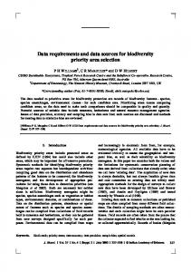
3.2 The STL format The STL format was developed by the Albert Consulting Group for 3D Systems in 1987, and it is currently the de facto industry standard for the transfer of part data to LM process planning systems [1][9][70]. The representation used for the 3D part model is a triangulated boundary representation. The format itself is a list of planar triangular facets, each triangle being defined by three distinct vertices and a normal direction pointing outwards from the interior of the object (see Figure 9) [1][70][98]. Since only the vertices are stored explicitly, the facet edges are represented implicitly. The ordering of the vertex data is significant, as will be seen later. The STL file format includes both an ASCII and a binary version, which are in fact not fully compatible. The rarely used binary version can transfer additional attribute information, but most LM systems cannot interpret it. Consequently, the ASCII version is used for most production purposes. 3.2.1 Advantages of the triangulated boundary representation and the STL format • Easy conversion: The STL format is very simple as it contains only a list of planar triangles. The conversion of a 3D model to the triangulated boundary representation uses standard surface triangulation algorithms. These are simple, robust and reliable when compared to algorithms for generating other types of approximations (such as general polygonal approximations). Also, the accuracy of the output can easily be controlled, and the possible types of degeneracy are few. • Wide range of input: Most 3D representations can be converted to a triangulated boundary representation due to the wide applicability of the available surface triangulation algorithms. This advantage is absent in most other approximation schemes. • Simple slicing algorithm: The algorithm for slicing a triangulated boundary representation is usually simple (but not necessarily efficient) as it only involves processing a list of triangles. All operations on a triangle can be made simple and accurate.

25

V1

N V3

V2 STL ASCII FORMAT FORMAT FOR EACH FACET solid

facet normal Ni Nj Nk

List of Facets

outer loop

endsolid

vertex V1x V1y V1z vertex V2x V2y V2z vertex V3x V3y V3z endloop endfacet Figure 9. The STL format

• Ability to split models: If the buildspace/workspace of the LM machine is small, the object model must be split into parts that individually fit into the buildspace. This is easily achieved for a triangulated boundary representation. However, each component must then be validated as an STL model in its own right. Note that all the advantages of STL arise from the use of a triangulated boundary representation of the object, and from the fact that the triangle is the simplest convex polygonal shape. Because of these advantages, STL is often used as a format for storing boundary information internally in the process planning system, in addition to its use for model transfer. 3.2.2 Disadvantages of the triangulated boundary representation and the STL format Despite the above mentioned advantages, three types of problems commonly occur with STL: (i) those caused by the triangulated boundary approximation, (ii) those related to the format itself, and (iii) those related to data conversion and transfer algorithms [9][66][67][68][70][76][98]. These are discussed in turn below.

26

(i) Problems intrinsic to the triangulated boundary representation: • Approximation: A major problem with the triangulated boundary representation is that curved surfaces can only be approximated by triangular facets as shown in Figure 10. A large number of facets gives a high approximation accuracy, but results in an extremely large amount of data. A smaller number of facets allows for less data but lacks accuracy.

Figure 10. STL approximation of a curved surface.

(ii) Problems intrinsic to the STL format: • File size: STL file sizes are unnecessarily large because of redundancy in the file format. Facet normal information is redundant, since the semantics of the representation allow this to be calculated from the ordered vertex list of each facet. Also, the great majority of vertices are multiply specified in the file, since they belong to more than one facet. It would be more efficient to specify each vertex once and make reference to it from each owning facet. This would also solve the problem of mismatched locations of vertices that are logically identical. • Truncation errors: The vertex coordinates and normal components of each facet are represented by single precision real numbers, their actual values being truncated. With the absence of topological information in the STL format truncation errors become significant, especially when the object is located far from the origin. A related point is that the object must be located in the positive octant, i.e., all coordinates are required to have positive values. • Incompleteness: The STL format incompletely describes the triangulated boundary representation because topology information is not stored. If it were present, this information could be used to speed up process planning tasks such as slicing. • Inconsistency: An STL file may have inconsistent tolerance values if it is created by appending two different STL files. Also, there may be gaps at the intersection of the two appended STL models.

27

• Inconsistent normals: Facet normals may be flipped (Figure 11) and thus be inconsistent with the orientation of other facets. Flipped surface normals may occur when surfaces are improperly defined in the original representation. • Incorrect normals: Explicitly specified facet normals may differ from the normals computed from facet vertices. This may be due to errors in the conversion algorithm.

Correct normals

Flipped normals

Figure 11. Flipped normals in some facets

(iii) Problems in conversion to the triangulated boundary representation: • Gaps: Surface facets (triangles) connect to form a set of closed shells that enclose or exclude material. If any facet is missing, then the shell is punctured, leaving a gap, and there is then no clear distinction between the inside and the outside the object. When a faceted model with gaps is sliced, the slices contain non-closed contours, and scan path vectors may extend beyond the boundary of the desired object (see Figure 12 and Figure 13). Gaps may occur because surfaces are missing in the original representation or because the vertices of a node shared by two or more facets are not the same for all facets due to truncation errors. Non-ideal modeling practice by CAD system operators is often responsible. • Internal walls: These may be generated by faulty geometric algorithms for closing gaps in a faceted model, or by imperfect user practice in constructing surface models. Internal walls may cause unsolidified boundaries between regions of material in the object as built (see Figure 14). • Degenerate facets: Facets may be degenerate, having zero area and therefore no defined surface normal. There are two kinds of facet degeneracy (refer to Figure 15): Topological Degeneracy: Two or more vertices of a facet coincide. Since this does not affect the geometry or connectivity of other facets, the degenerate facet can be discarded. Geometric Degeneracy: All the vertices of a facet are distinct, but they are collinear. Such a facet has no normal, but it contains implicit topological information on the connectivity of neighboring facets, and may not be discarded. 28

Gaps

Surface 2

Surface 1

Figure 12. Gaps due to missing facets.

Stray vectors with no endpoints

Contour of a slice

Fill pattern

Figure 13. Stray vectors due to missing segments of a contour • Incorrect intersections: Facets may intersect at incorrect locations (apart from at their edges), giving rise to interpenetrations (see Figure 16). Much time and effort is currently spent in correcting faulty STL files and generating topological information from the facets [69][70][71][72][73][74][75][76][77][78][79]. It has been estimated that about 10% of STL files formed from solid models have flaws, while 90% of those formed from surface models exhibit problems [80]. Often, corrections made to the STL file, necessitated by missing or redundant surfaces in the surface or solid model of the part, are not

29

Internal walls Figure 14. Internal walls due to improper joining of objects

Geometric Degeneracy A degenerate triangle with three unique vertices

Topological Degeneracy A degenerate triangle with three coincident vertices – a point A degenerate triangle with two coincident vertices – a line

Figure 15. Degeneracies in STL format

30

Figure 16. Non-boundary intersection of two triangles passed back to the designer for correction in the original shape model. If further design refinements or changes are made by the designer and another STL file is generated and transmitted to the manufacturer, it is therefore likely that the same facet corrections will need to be made yet again before process planning can continue [81].

3.3 Alternatives to STL The STL format was apparently adopted because robust, easily used surface triangulation schemes were already available within most CAD systems when LM was being developed. The initial application of LM was rapid prototyping, i.e., the quick creation of physical mock-ups for design verification. In this context, approximation of the 3D boundary of the object and the use of the STL format proved adequate. Most LM process planning algorithms, having been developed after the development of the STL format, use STL models for importing 3D boundary geometry from various commercial CAD systems. For this purpose, STL therefore plays the role of a neutral format as defined earlier. Thus, having originally been adopted as a proprietary format by the earliest LM system provider, the STL format eventually became a de facto industry standard. Over the last decade, significant advances have been made in all aspects of LM technology, including hardware, software and materials. New materials and process capabilities have expanded the application domain of LM beyond rapid prototyping to the manufacture of tooling, and to the production of one-off or short run functional parts. Consequently, the nature of the information transmitted to the LM process planning system has become more critical. For example, as was shown earlier, the automation of process planning algorithms ideally requires more accurate geometrical information than is provided by STL, together with topological and process information. Further, selective deposition of material for the creation of heterogeneous structures requires material information in the object model. Such requirements cannot be met by the triangulated boundary representation of the purely geometric STL format. These facts, together with the drawbacks of the STL format described in Section 3.2.2, provide the motivation for developing alternative input formats for LM process planning systems. Clearly, any new LM data transfer format must continue to contain a representation of the 3D part boundary, though not necessarily as a triangulated approximation, and it should desirably include representations of other data such as material property distribution within the object, surface attributes, process parameters, etc. The following subsections survey the various alternatives to the STL format that have been proposed in the literature.

31

3.3.1 STH − Surface Triangles Hinted format The STH format was developed by Brock Rooney and Associates. It uses a triangulated boundary representation, with flexible rules for efficient storage of vertex and connectivity information [1]. It is more compact than STL, and contains optional structural information on source volumes and surfaces. Hence, the underlying representation used by STH is similar to that of STL, but the chosen format requires less storage, and the provision of connectivity information allows the use of more efficient slicing algorithms. 3.3.2 CFL − Cubital Facet List format The CFL format was developed by Cubital [82][83] to overcome the problems with STL, but has not become very popular. It defines a general planar-faceted polyhedral boundary representation, in which facets may contain multiple polygonal holes. The coordinates of all the vertices are stored and indexed. The facet descriptions reference the vertices by their indices and not by value. This saves space and also implicitly captures the connectivity relations between facets in the model. The format also has provisions for storing textual comments, and, unlike STL, allows for the alternative description of a model as a series of contour slices. Apart from this extension beyond the STL capability, the availability of topological information in the model has advantages as previously noted. 3.3.3 RPI (Rensselaer Polytechnic Institute) format The RPI format [84] describes both faceted boundary representations and CSG models defined in terms of Boolean operations on primitive volumes. The format allows the specification of 3D transformations, multiple instancing of model elements, and process parameter values. It defines a set of entities in terms of schemas, and the data is logically subdivided into records composed of fields. A record is an instance of a schema-defined entity, and record fields have specified variable types (integer, float, double, string, boolean and n-bit binary). In the simplest case, this format defines vertices and faces. An indexed list is created of all vertices occurring in the boundary of the object, and the face list then directly references the vertices by their indices in the vertex list. The RPI format also allows more complex representations to be captured, including CSG models as mentioned earlier. This format therefore has the flexibility to define and store entities in different ways, and its capabilities subsume those of the STL, CFL and CSG formats from the shape modeling point of view. It has the added advantage of storing process information. 3.3.4 STEP – Standard for the Exchange of Product Data STEP, or more formally ISO 10303 [85][101], is an international standard for the exchange of product life-cycle data, where life-cycle is broadly interpreted to include design, analysis, manufacture, maintenance and disposal. The STEP standard has built on experience gained with earlier computer graphics and product data transfer standards, and its scope is continually expanding to cover new classes of products and new phases of the product life-cycle. It goes far beyond the pure shape aspect of a product to include administrative, material, product structure and manufacturing information. At present, STEP is most highly developed in the area of mechanical products, but it is intended eventually to cover a very wide range of discrete industrial products, from

32

microelectronics to cars and ships. Its scope excludes the products of the process industries, though the facilities for their production may be regarded as discrete products in their own right, and there is a growing interest in the process plant area. In order to make the STEP standard as clear, unambiguous, and extensible as possible, a three layer architecture has been adopted. Data specifications are divided into conceptual, application and physical layers. The conceptual layer, known in STEP as Integrated Resources (IRs), contains sets of related data entities that can be specialized to describe different domains of interest. For example, one IR (Part 42 – Geometrical and topological representation [104]) contains entities for describing the geometry and topology of an object. The STEP IRs are the basic building blocks for defining neutral file formats to capture the data for particular life-cycle stages of particular types of product. This is done in the application layer, where subsets of the IR data entities are defined and specialized for the desired purpose. This results in a series of Application Protocols (APs) that prescribe the scope and representation of the data that can be exchanged for that purpose. For instance, Application Protocol AP203 (Configuration controlled design) [109] specifies the means for exchanging mechanical engineering design data between computer aided design (CAD) systems. The third (physical) layer of STEP architecture defines how the data elements are mapped into a physical file format (Part 21) [102] or how it may be accessed in a data repository (Part 22) [103]. Several research groups have suggested using STEP for the transfer of data to LM process planning systems [6][86][87][88][89][98]. In [88], the author points out the need for the product model to be used in selecting process parameters and in planning tool paths, and suggests an extension of STEP AP204 (Mechanical design using boundary representation) [110] to include information on process parameters, scanning patterns and material data. STEP models could also contain the results of build simulations and analyses on how different scan strategies will affect the final part. This information could be used by the process planning software to select final values of the build parameters. A STEP-based transfer of design data (in this case the geometry of the part) to an LM process planning system has been demonstrated in [89]. Using software tools already available in the marketplace, a Brep solid model of a part is translated into STEP AP203 form for transfer to the process planning software. There the part geometry is converted into the software's faceted boundary representation internal format, and the LM data is generated and sent on to the fabrication device. An AP specific to LM has not yet been developed, but the STEP IRs appear to provide adequate means for this to be done. To be specific, Part 42 defines geometrical and topological facilities that allow the capture of geometric models of several different types. These include manifold surface with topology, faceted boundary representations, simple and advanced Breps with curved surfaces (differing in whether or not they allow the use of NURBS surfaces) and CSG models. Groupings of basic capabilities called Application Interpreted Constructs (AICs) are defined for each of these model types, and they can be used as ready-made building blocks in the construction of new APs. The AICs concerned with shape representation are already in use in AP202 [108] and AP203 [109], two of the four APs that have so far reached international standard status, and are therefore readily available for use in any new proposed AP. To give a little more detail of one of these APs, AP203 defines the data requirements for the exchange of information between CAD systems, e.g., between Unigraphics and AutoCAD, a common type of requirement in manufacturer/supplier situations. APs are divided into Units of Functionality (UoFs), which are groups of functionally-related data entities. In AP203, the UoFs can be further classified as those that pertain to design management, and those that pertain to the shape of the object. Within design management the UoFs are authorization, bill of material, 33

design activity control (relating to part versioning), design information (material and process specifications, surface finish), effectivity (time and batch number constraints on a part in the product), end item identification (configuration of final parts), part identification, and source control (suppliers). The shape UoF allows the following representations: wireframe with topology, manifold surface with topology, non-topological surfaces and/or wireframes, faceted boundary representation, or advanced boundary representation solid (having curved surfaces). An AP for LM would not necessarily need all of these UoFs, but it would certainly need to include at least one of the existing AICs defining model types in the shape UoF, to allow the transfer of the part model – it may be noted that the AIC for faceted boundary representations provides a capability encompassing that of STL, but including topology and excluding the redundant surface normal information. The wireframe AIC could also be used, to capture slice contours. Part 45 of STEP [105] is an IR providing facilities for the capture of material properties, and this would need to be used since material data is one of the requirements identified for LM process planning. Similarly, other IRs could be called upon for the transfer of process-related data [106] and tolerance information [107]. 3.3.5 Discussion Of the proposed alternatives to STL, STH improves on STL by storing more information and using better storage schemes. CFL, RPI, and STEP can all transmit general polyhedral models in addition to triangulated models. However, as mentioned above, the use of a polyhedral part model has inherent drawbacks. The STEP and RPI formats can transmit exact geometry and process information, both outside the capability of CFL, STH, or STL. STEP has the added advantage that it can handle material and tolerance data. Further, its basic IRs and some APs have already gone through international standardization procedures and have been extensively tested in practical data exchange. By contrast, the RPI format does not have the same scope or standard status, and has certainly not been tested to the same extent. In Section 3.6, we evaluate these formats in further detail. It should be mentioned that other formats have been developed by various commercial CAD companies for transfer of data to and from their systems. Such formats would need to be extended for use in the LM context, and none of them appears to offer any advantages over the formats already discussed. The same holds for the US national CAD data exchange standard IGES (Initial Graphics Exchange Specification)[100], which is currently widely used but destined to be replaced by STEP in the foreseeable future.

3.4 Slice Formats for LM After the 3D object model is transferred to the process planning software, it is sliced to generate the layer information, as described in Section 2.1.6. In the following, we analyze the role of slice formats in LM process planning and present some of the proposed formats that could serve as a standard. A slice format must enable the storage of all the geometrical data of the layer, including the layer thickness. Also, it must have provision to store material and process-related information, if necessary. A typical slice geometry is shown Figure 17. Currently, there is no standard format for slice data. Often the LM user never encounters this data in a physical file because it is generated and stored internally in the process planning soft-

34

Material Internal Contour

External Contour

Figure 17. A typical slice ware. However, to exchange slice information between process planning systems, a standard slice format is required. Some of the proposed slice formats are described below. 3.4.1 CLI − Common Layer Interface CLI, whose development started in a European BRITE/EURAM project [90], is aimed at providing a simple, efficient and unambiguous slice format for data input to all LM systems. Each layer is represented by its thickness and a set of contours. Contours define the boundaries of the solid material within a layer and are represented by polylines. Each contour should be closed and have no intersections with itself or with other contours. A hatch is also defined, as a set of independent straight lines each defined by a start and an end point. Hatches are used with open polylines to define support and filling structures. Polylines representing internal contours are ordered clockwise and those of external contours counterclockwise when viewed along the negative Z-axis. No non-geometric information is defined in CLI. Although development was commenced by a group of automotive companies, the current version of CLI has been enhanced through collaboration with a second BRITE/EURAM project for use with medical scan data. 3.4.2 LEAF − Layer Exchange ASCII Format Development of LEAF was started by Helsinki University of Technology in another BRITE/ EURAM project [91], and it has also been worked on by the Fraunhofer Institute IPA in Stuttgart [92]. The format consists of two sections − a header section and a geometry section. The header section contains preprocessing information, including keyword definitions and vendor or machine-specific information. It also specifies mathematical information necessary for the proper interpretation of the geometry section (such as the radix of the number system used, units and ranges of values) and technological information defining the structure of hatches and supports. The header data can be directly referenced from the geometry section rather than being explicitly restated each time it is needed. The geometry section contains the layer-based geometrical data of the part model. The upper-level layer entity used contains both geometry and process data, and it can have sub-entities such as regions, contours, hatches, supports etc. Each contour is a non-self35

intersecting polygon described in terms of 2D primitives, the polyline and the circular arc. 3.4.3 HP-GL − Hewlett Packard Graphics Language HP-GL is a 2D plotting language developed by Hewlett Packard for use with plotters and printers [93]. It comprises a core set of instructions, called the HP-GL kernel, together with several device-specific extensions. The kernel contains most of the plotting instructions, which fall into five functional groups: configuration and status, vector, polygon, line and fill attributes, and character. Each HP-GL instruction has four components: a mnemonic, parameter(s), separator(s), and a terminator. Since HP-GL is capable of representing arbitrary 2-D shapes with any fill pattern, it can be used to represent slices and can also be used to drive an LM machine. 3.4.4 SLC formats Various LM system vendors have developed proprietary slice formats. Although they differ, they are all generally referred to as SLC formats. Without exception they use polyline approximations to represent slice contours. One example is the SLC format used by the Stratasys FDM 3-D Modeler [94]. 3.4.5 STEP Although no one has yet demonstrated the use of STEP to transfer slice data between LM process planning systems, the resources are available within this standard for doing so. The STEP Integrated Resources, specifically Part 42 (Geometric and topological representation) [104] contain all that is needed for defining contours and fill patterns. For contours, polyline approximations are available, and exact geometry including NURBS curves could also be used if desired. It would be relatively easy to develop an LM-specific Application Protocol using these shape modeling resources and the capabilities for capturing materials information defined in Part 45 [105]. Both the geometry and the materials resources are already parts of the international STEP standard ISO 10303. Process information could also be included by using Part 49 (Process structure, properties, and representation) [107]. 3.4.6 Discussion As mentioned earlier, there exists no industry standard for 2D slice data to supplement the almost universal use of STL for 3D models. As evidenced by some of the proposals described above, there is a need for such a format to provide a common basis for communicating layer information. This will not replace the 3D format if current practice continues to be used, since the 3D information provides input to the slice generator while the slice format captures its output. Of the above mentioned slice formats, LEAF and STEP are the most complete since they provide the means for transmitting additional information beyond geometry. HP-GL could also be completed by the addition of a LM-specific extension to include process information. We evaluate these formats in further detail in Section 3.6.

36

3.5 Motivation for alternate 3D representations Despite the remark made in the last paragraph, the establishment of a standard slice format has been considered by some as an actual replacement for STL [67][95]. Such a departure from current methods would imply that slicing is performed prior to input of data to the LM system rather than in that system itself, as is usually the case at present. The suggested reasons for jettisoning the 3D format include the following: • The CAD model could be analyzed directly to determine a good build direction and the required support structures. Then it could be sliced. Alternatively, the CAD model could be sliced first, and the support structures created by analyzing the slices. These operations could be performed using native capabilities of the CAD system concerned. • CAD models based on precise geometry representation (such as NURBS-based Brep) could be used to represent slice data without the loss of precision inherent in STL. Hence, direct slicing of such models can give parts with improved surface finish. It may also lessen the time needed for process planning, since in order to achieve similar accuracy using STL a fine level of discretization must be used in generating the STL file. This results in a very large file and increases the chances of numerical problems in the triangulation and slicing algorithms. • CAD systems could take advantage of their proprietary capabilities to optimize the slice algorithm and validate the results. This would avoid the generation of an STL file and the possible need to correct errors in it before transfer to the LM system. • The entire data storage requirement of the STL file would be eliminated. • In most cases, correction of faulty geometry is easier and quicker in sliced data. • A slice data format may be more viable for use with parts defined in terms of scanned or image input data, since it avoids the necessity to create a full 3D solid model, which is a difficult task. The above mentioned advantages are not intrinsic to the slice format itself, but arise mainly from the drawbacks of triangulated boundary representations (e.g., STL) and the current need to convert into that form from other representations. What the preceding points suggest is that the initial input to process planning should not be a triangulated boundary representation, but some format more closely related to the original part data, i.e., an exact CAD model or a set of digitized data points. This would obviate the need for a 3D model transfer in cases where slicing is performed directly in a CAD or other external system, but that 3D capability needs to be retained for other cases in the interests of flexibility. Two disadvantages in completely abandoning a 3D transfer format in favor of a slice format are the following: • Once the model is sliced, ability to manipulate the model and change build orientation in the LM system is lost. One implication here is that it is preferable to slice the model immediately before fabrication. • Although most current LM technologies fabricate parts in layers, there are freeform fabrication techniques in which material is deposited in 3D. Such methods clearly demand some approach other than slicing, but that approach could also be based on original model data rather than an intermediate STL or other triangulated model. On the basis of the considerations given in this section, we recommend the adoption of an advanced boundary representation of a part as input to process planning for LM. This may be oriented and sliced in the originating CAD system, but a neutral format must be provided for the 3D representation to provide for cases where this is not done. A standard format for slice data is also

37

needed, to allow the transfer of slice representations, either between an originating CAD system and a LM process planning system, or between different LM systems.

3.6 Comparison of 3D and slice formats In this section we specify what are the most important requirements, in our view, for neutral exchange of data in the context of LM. We then compare the various 3D and slice formats described in earlier sections of this paper against these requirements. Table 2 and Table 3 show the representations and their corresponding formats, as surveyed in this report, for 3D data and slice data respectively. Table 4 shows a comparison of 3D shape formats, while slice formats are compared in Table 5. Table 2. Representations and corresponding formats for 3D design data Representation

Format(s)

Triangulated boundary

STL, STH, CFL, RPI, STEP

Faceted boundary

CFL, RPI, STEP

General surface

various vendor specific formats, STEP

Brep solid

various vendor specific formats, STEP

CSG solid

various vendor specific formats, RPI, STEP

Points

none proposed for LM (usually converted to alternate representation)

Images

none proposed for LM (usually converted to alternate representation)

Mathematical

none proposed for LM (usually converted to alternate representation)

Table 3. Representations and corresponding formats for slice data Representation

Format(s)

Polyline contours

CLI, LEAF, HP-GL, SLC, STEP

Straight line and circular arc contours

LEAF, STEP

Parametric curve contours

STEP

Our choice of metrics in the two tabular evaluations reflects the requirements we consider important for a neutral format. Most of these metrics relate to properties of representation schemes [8] and neutral exchange formats [96], and we believe that they provide a useful set of guidelines for our present purpose. We list below all the metrics used in Table 4 and Table 5, with brief explanations, grouped under the headings “Neutral Exchange Format Issues” and “Secondary 3D Representation Issues”. Neutral Exchange Format Issues: • Completeness: The neutral format must capture all the information necessary for LM fabrication of the part that is present in, or can be derived from, its primary CAD model. • Neutrality: The exchange format must be independent of the sending and receiving systems, and of the representational nature of the initial part model.

38

• Efficiency: The format must be concise and hence economical in its storage requirements. • Extensibility: The format should have the flexibility to allow definition of new entities, so that its domain can be expanded to meet future needs. • Ability to inspect: The neutral format must be suitable for inspection and verification. • Robustness: The neutral format should not be prone to errors. • Compatibility: The underlying representation used should allow simple mappings from CAD or other input models to ensure that translation is not too computationally intensive. • Breadth of domain: This is related to Completeness above. The Domain field in the tables below indicates the specific types of data that can be stored by the format concerned (e.g., geometry, topology, material, process, tolerances, etc.). Secondary 3D Model Representation Issues: • (Representation) Type: This field in the table specifies the representation scheme(s) each format can store. • Accuracy: The representation should not approximate the object unless such an approximation is found sufficient by the user for the task in hand. • Efficiency: The representation should allow the use of a model format permitting efficient data retrieval and manipulation. • Redundancy: The representation should not store excessive redundant information. Some redundancy may be found desirable to allow efficient processing of the file, but this clearly impacts storage requirements. Such trade-offs are characteristic of modeling representations. • Repairability: The correction of errors in the model representation that arise during the data transfer due to roundoff and related causes must be easily and quickly repairable. The evaluations made in Table 4 and Table 5 are based on the information presented earlier. We have chosen not to include IGES [100] or DXF. The first is a widely used US standard CAD data exchange format originally designed to handle drawings, 3D wire frame and surface models, though provisions for exchanging CSG and Brep data have more recently been added. However, STEP improves upon IGES in many respects [97], and when the final release of IGES (Version 6) is made a migration plan will be implemented enabling IGES users to move gracefully to the use of STEP. DXF, also widely used, is an unpublished model transfer format from Autodesk Inc. Like IGES, it is also inferior to STEP in several respects, and since it is also proprietary it will be excluded from consideration here. It is reasonable to restrict our coverage of CAD transfer formats to STEP in this survey because • STEP is an international standard, easily extensible to cover the LM domain through the use of existing Integrated Resources, and • STEP will almost certainly ultimately supersede the older standards for CAD data exchange. However, we have included the G-WoRP format mentioned earlier because it is quite different from the others and offers an interesting comparison. All evaluations given in the tables are, of course, non-quantitative. The assignment of qualitative “grades” to the various formats is obviously a matter of opinion, but we have done our best to provide some support for our opinions expressed earlier in this survey.

39

Table 4. Comparison of 3D Exchange Formats ISSUES

PROPERTIES

STL

STH

CFL

RPI

G-WoRP

STEP

Completeness

No

No

No

Yes

Yes

Yes

Neutrality

Yes

Yes

No

Yes

No

Yes

Efficiency

B

B

F

G

B

F

Extensibility

B

B

B

G

B

G

Inspectibility

F

F

G

G

B

G

Robustness

F

F

F

F

F

F

Compatibility

G

G

F

G

B

G

Domain

GM

GM

GM, TP

GM, TP

GM

ALL

Type

TB

TB

FB

FB,CG

VX

TB, FB, BR,CG

3-D

Accuracy

F

F

F

F

F

F-G

Representation

Efficiency

B

B

F

F-G

B

F-G

Issues

Redundancy

B

F

G

G

G

G

Repairability

F

F

F

F

F

F

Neutral Exchange Format Issues

40

GM: Geometry Data TP: Topology Data PR: Process Data ALL: All data - GM, TP, and PR

G: Good F: Fair B: Bad

TB: Triangulated Boundary FB: Faceted Boundary BR: Boundary Representation CG: Constructive Solid Geometry VX: Voxels

Table 5. Comparison of Slice Formats ISSUES

Neutral Exchange Format Issues

41

2-D Representation Issues

PROPERTIES

CLI

LEAF

SLC

HP-GL

G-WoRP

STEP

Completeness

Yes

Yes

Yes

Yes

Yes

Yes

Neutrality

Yes

Yes

No

Yes

No

Yes

Efficiency

F

G

F

F

F

F

Extensibility

F

G

F

F

F

G

Inspectibility

G

G

G

G

G

G

Robustness

G

G

G

G

G

F

Compatibility

G

G

G

G

G

G

Domain

GM, TP

ALL

GM, TP

GM,TP

ALL

ALL

Type

PL

PL,CA

PL

PL

PL,PC

PL, CA,PC

Accuracy

F

G

F

F

F

G

Efficiency

G

G

F

G

G

G

Redundancy

G

G

G

G

B

G

Repairability

G

G

G

G

G

G

GM: Geometry Data TP: Topology Data PR: Process Data ALL: All data - GM, TP, and PR

G: Good F: Fair B: Bad

PL: Polylines CA: Circular Arcs PC: Parametric Curves

4.0 Conclusions Process planning for LM involves several tasks, each having specific data requirements, as summarized in Table 6. Various file formats are in use or have been proposed for transferring the necessary data between different stages of LM process planning. Although many of them are restricted to the exchange of geometry data, the table shows that other types of information also need to be transferred. A new neutral file format needs to be selected or developed for this purpose because the current de facto standard, the STL file, does not allow for the storage of nonboundary data. In the authors’ opinion, extension of the STL specification will not be a satisfactory long-term solution in view of the deficiencies of that format noted earlier. The STL format was initially developed to serve as an exchange format for the stereolithography process (the first commercial LM technology) and was not designed to serve as an industry standard. Nevertheless it has served industry well in the early years of LM technology, since from the outset its triangulated representation has been reasonably compatible with the representations used by most CAD systems, including some whose CAD models were themselves faceted in the late 1980s. If the LM domain were to remain that of “design verification” and success were achieved in the generation of error-free STL files, or at least their automated repair, the triangulated boundary representation could continue to serve quite adequately. There would in this case be no virtue in replacing it with some other format. However, the question of whether the triangulated boundary representation needs to be replaced must also be viewed in the context of the future potential of LM. Some particular aspects that need consideration here are • The prospect that LM techniques will become suitable for production use (apart from their current applications for molds and dies) in the medium-term future. This will place a premium on the transfer of exact product geometry from the CAD system, together with information on tolerances, surface finish and materials. • The prospect that some phases of LM planning will migrate into the CAD system, raising the need for a standardized slice format. • The prospect of using LM for the generation of parts with embedded electronic or other components, multi-material parts or parts in which the material properties vary continuously or exhibit non-isotropy . These will require completely new capabilities in LM data transfer. The last point merits some explanation. The technology is already available for selective deposition of materials on a given layer. Multi-material structures can therefore be manufactured. Furthermore, current hardware and material research in LM is aimed at developing the capability to deposit materials with variable composition and/or embedded fiber reinforcement [111]. In this context, it may be noted that recent advances in structural and material design can yield optimal product shapes having inhomogenous material distributions. Thus one missing capability in this product design and layered manufacturing environment is a means for representing a 3D CAD model with material inhomogeneity and/or non-isotropy in its solid interior. When this becomes possible, we will need a 3D LM data transfer format with corresponding capability, and a matching slice format that can capture appropriate scan strategies. The use of voxels with attributes is a possibility, but would have the disadvantages pointed out in Section 2.3. The materials issue is potentially of fundamental importance, and research is needed for the development of enhanced 3D representation schemes incorporating materials data, leading in turn to standardized 3D model and slice formats that contain full material type and property information for LM.

42

Table 6. Process planning data requirements, their representations, and formats Input Data

Representations

Formats

Task

Boundary

Triangulated boundary

STL

Orientation

STH

Support structure design

CFL

Slicing

RPI STEP Brep

STEP

CSG

RPI STEP

Slice

Polyline

CLI

Path planning

LEAF HP-GL SLC STEP Polyline with circular arcs

LEAF STEP

Material

Parametric curves

STEP

Structured attribute

STEP

Orientation Slicing Path planning

Surface finish

Attribute

STEP

Orientation Slicing Path planning

Tolerances

Structured attribute

STEP

Orientation Slicing Path planning

Process data

Structured attribute

RPI

Orientation

STEP

Support structure design Slicing Path planning

Our comparison of the various 3D and slice formats proposed for LM, and the summary of process planning tasks and their required data inputs shown in Table 6, lead us to recommend the development of a STEP AP specifically for the purpose of LM process planning. STEP resources already exist for handling most of the different types of data identified in this survey as required for LM process planning, including process parameters, tolerance and surface finish requirements. The 3D shape data can be transferred using the STEP faceted boundary representation (a direct 43

replacement for STL), or better, as an advanced Brep solid containing topology information and having general curved surfaces. STEP also allows for the representation of CSG solids, though few process planning applications accept this kind of input. In addition to 3D models, STEP resources can be used to represent slice contours in terms of polylines, circular arcs, conic segments or free-form parametric curves. The one major required capability lacking in STEP is that for modeling inhomogeneous materials, but a resource that can be used for this purpose is currently under development. The wide choice of possibilities available could be categorized by the definition of Conformance Classes, such as have been devised for existing STEP APs. For example, a Conformance Class 1 could be specified that provides almost exactly the capabilities currently available in STL, while other classes could contain a wider range of information and/or use more sophisticated part representations. As with all STEP APs, compliance of translators with their specified conformance classes would be subject to stringent testing by independent bodies. To summarize, we have chosen the STEP standard for several reasons. Firstly, it allows the most flexibility in choosing an appropriate representation for the data that needs to be transferred to the process planning system. Both 3D and slice data would be defined within the context of the same standard, which simplifies the standardization procedure. Secondly, STEP already has the necessary resources for representing the material, tolerance and process data needed for LM process planning. Thirdly, as can be seen from Tables 3 and 4, the STEP standard satisfies reasonably well the key features sought in a neutral file format, as discussed in Section 3.6. Finally, many of the existing STEP IRs and APs are already components of an international standard that is increasingly used by industry. Several of the capabilities needed for the new AP already exist, have been tested and refined in practical use, and can be adopted wholesale in the form of Application Interpreted Constructs (AICs). We believe that these considerations provide strong support for our recommendation.

5.0 Acknowledgments This report is an amalgamation and extension of two previously published papers1. The authors recognize the support of the NIST SIMA and DARPA RaDEO projects.

1. References: Marsan, Anne, and Dutta, Deba. “A survey of process planning techniques for layered manufacturing”, Proceedings of the 1997 ASME Design Technical Conferences, Sacramento, CA, 1997. Kumar, Vinod and Dutta, Deba. “An Assessment of Data Formats for Layered Manufacturing”, Advances in Engineering Software, 28, 3, 151-164, 1997.

44

6.0 Addendum - Recent developments The National Institute of Standards and Technology (NIST) has been taking an interest in layered manufacturing as an emerging technology for several years. A state-of-the-art report was published in 1993 [98], but until recently NIST has not pursued any LM-related standards activity. However, this report makes it clear that the time is now ripe to embark on such an activity, since the current de facto LM standard is increasingly seen as inadequate for the future. NIST has recently held two workshops, with participants from industry, academia and government, to discuss the way forward in standards for LM. The proceedings of these workshops are currently being prepared for publication, but in the meantime a white paper was written after the second of them, to serve as a consultative document [99]. As far as informational standards are concerned, this recommends two approaches, one for the short term and one for the longer term. The first recommendation is that STL be extended so that it can transfer a wider range of information. The second is that, as suggested in this report, the resources of ISO 10303 (STEP) should be used as the basis for an extensible long-term LM standard. The intended outcome of the NIST work (and also related work in some other organizations) is sometimes informally referred to as SIF (Solid Interchange Format). However, it is unlikely that this name would persist within the context of STEP, which already provides general-purpose representations of solid shapes. As a separate development, the first meeting of a STEP Rapid Prototyping Interest Group was held in Bad Aibling, Germany, in June 1998. The initial impetus for the meeting came from Canada and Japan, but representatives from several other countries were also present. These included two participants from NIST. It was agreed to hold further such informal meetings on a regular basis, with the aim of initiating a new formal STEP activity in the LM area once the scope of the new work has been agreed. NIST will press for the inclusion of the material, tolerance and process information mentioned earlier in this report.

45

7.0 Glossary of Acronyms Where appropriate, page references are given to the first mention of the acronym. In some cases a further reference to a full description is provided. 2D – two-dimensional 3D – three-dimensional 3DP – Three Dimensional Printing (p. 4) AIC – STEP Application Interpreted Construct (p. 46) ANSI – American National Standards Organization AP – STEP Application Protocol (p.45) Brep – Boundary representation (p. 9) BRITE – Basic Research in Industrial Technology for Europe (p. 49) CAD – Computer Aided Design (p. 9) CD – Committee Draft (of ISO standard) (p. 73) CFL – Cubital Face List (p 44) CLI – Common Layer Interface (p. 49) CMM – Coordinate Measuring Machine (p. 10) CSG – Constructive Solid Geometry (p. 9) CT – Computerized Tomography (p. 11) DARPA – Defense Advanced Projects Research Agency DFLM – Design for Layered Manufacturing (p. 26) DIS – Draft International Standard DMD – Direct Metal Deposition (p.4) DXF – Drawing eXchange Format (p. 55) EURAM – EURopean Applied Materials program (p. 49) FDIS – Final Draft International Standard (pp. 72, 73) FDM – Fused Deposition Modeling (p. 4) G-WoRP – Geometric Workbench for Rapid Prototyping (p. 27) HP-GL – Hewlett-Packard Graphics Language (p. 50) IGES – Initial Graphics Exchange Specification (p. 55) IR – STEP Integrated Resource (p. 45) ISO – International Organization for Standardization LEAF – Layer Exchange ASCII Format (p. 49) LM – Layered Manufacturing (p. 2) LOM – Laminated Object Manufacturing (p. 4) MRI – Magnetic Resonance Imaging (p. 11) NIST – National Institute of Standards and Technology NURBS – Non-Uniform Rational B-Splines (p. 9) RaDEO – Rapid Design Exploration and Optimization (p. 61) RP – Rapid Prototyping (p. 4) RPI – Rensselaer Polytechnic Institute (p. 44) SDM – Shape Deposition Modeling (p. 5) SIF – Solid Interchange Format (p. 62) SFF – Solid Freeform Fabrication (p. 4) SGC – Solid Ground Curing (p. 4) SIMA – Systems Integration for Manufacturing Applications (p. 61) 46

SLC – one of several different proprietary layer data formats (p. 50) SLS – Selective Laser Sintering (p. 4) STEP – STandard for the Exchange of Product model data (pp. 7, 44, 50) STH – Surface Triangles Hinted (p. 43) STL – a file format, originally intended for stereolithography (pp. 7, 34) UoF – STEP Unit of Functionality (p. 46)

47

8.0 References 1.

Burns, Marshall. Automated Fabrication. Englewood Cliffs, NJ: Prentice Hall, 1992.

2.

McMains, Sara Anne. Rapid Prototyping of Solid Three-Dimensional Parts, Master’s Project, University of California, Berkeley, CA, 1995.

3.

Mazumder, J., Koch, J., Nagarthnam, K., and Choi, J. Rapid Manufacturing by Laser Aided Direct Deposition of Metals, Technical Report, University of Illinois, Department of Mechanical Engineering, 1996.

4.

Bendsøe, M. P. and Kikuchi, N. “Generating Optimal Topologies in Structural Design using a Homogenization Method”, Computer Methods in Applied Mechanics and Engineering, vol. 71, 1988, pp. 197-224.

5.

Bendsøe, M. P., Diaz, A. and Kikuchi, N. “Topology and Generalized Layout Optimization of Elastic Structures”, Topology Design of Structures, M. P. Bendsøe and C. A. MotaSoares, eds. Amsterdam: Kluwer Academic Publishers, 1993, pp. 159-205.

6.

Kochan, D. Solid Freeform Manufacturing. Amsterdam: Elsevier, 1993.

7.

Dolenc, A. Rapid recipes for parametric surface models. Technical Report, Helsinki University of Technology, 1994.

8.

Requicha, A. “Representations for Rigid Solids: Theory, Methods and Systems”, Computing Surveys, vol. 12, no. 4, 1980, pp. 437-464.

9.

Pacheco, Joselito M. State of the Art Review: Rapid Prototyping for Manufacturing. Technical Report MTIAC SOAR-93-01, IIT Research Institute, March 1993.

10. Marsan, A. and Dutta, D. “Construction of a CAD Model from 3D Homogenization Output”, Proceedings of the Design Engineering Technical Conferences, vol. 1, ASME, 1995, pp. 133140. 11. Sreeram, Puduhai N. and Dutta, Debasish. “Determination of Optimal Orientation Based on Variable Slicing Thickness in Layered Manufacturing,” Proceedings of the 1995 ASME Winter Annual Conference, San Francisco, CA, Nov. 1995. 12. Bablani, Minoo, and Bagchi, Amit. “Quantification of Errors in Rapid Prototyping Processes, and Determination of Preferred Orientation of Parts,” Transactions of the North American Manufacturing Research Institution of the SME, vol. XXIII, SME, Houghton, MI, May 1995, pp. 319-324. 13. Cheng, W., Fuh, J. Y. H, Nee, A. Y. C., Wong, Y. S., Loh, H. T., and Miyazawa, T. “Multiobjective optimization of part building orientation in stereolithography,” Rapid Prototyping Journal, vol. 1, no. 4, 1995, pp. 12-23. 14. Allen, Seth and Dutta, Deba. “On the Computation of Part Orientation Using Support Structures in Layered Manufacturing,” Solid Freeform Fabrication Symposium 1994, H. L. Marcus et al., eds., University of Texas, Austin, 1994, pp. 259-269. 15. Frank, Dietmar and Fadel, Georges. “Preferred Direction of Build for Rapid Prototyping Processes,” Proceedings of the Fifth International Conference on Rapid Prototyping, R. P. Chartoff, A. J. Lightman, and J. A. Schenk, eds. University of Dayton, June 1994, pp. 191-200.

48

16. Frank, Dietmer and Fadel, Georges. “Expert system-based selection of the preferred direction of build for rapid prototyping processes,” Journal of Intelligent Manufacturing, vol. 6, no. 5, October 1995, pp. 339-345. 17. Thompson, David C. and Crawford, Richard H. “Optimizing Part Quality with Orientation,” Solid Freeform Fabrication Symposium 1995, H. L. Marcus et al., eds. University of Texas, Austin, August 1995. 18. Suh, Yong S. and Wozny, Michael J. “Integration of a Solid Freeform Fabrication Process into a Feature-Based CAD System Environment,” Solid Freeform Fabrication Symposium 1995, H. L. Marcus et al., eds. University of Texas, Austin, August 1995. 19. Jacobs, Paul F. Rapid Prototyping and Manufacturing. McGraw Hill, New York, 1992. 20. Kirschman, C. F., Jara-Almonte, C. C., Bagchi, A., Dooley, R. L., and Ogale, A. A. “Computer Aided Design of Support Structures for Stereolithographic Components,” Proceedings of the 1991 ASME Computers in Engineering Conference, Santa Clara, CA, August 1991, pp. 443-448. 21. Webb, Douglas, Verdes, Victor, and Cassapis, Constantin. “Computer-aided Support-Structure Design for Stereolithography Models,” Proceedings of the Fifth International Conference on Rapid Prototyping, R. P. Chartoff, A. J. Lightman and J. A. Schenk, eds. University of Dayton, June 1994, pp. 221-228. 22. Swaelens, Bart, Pauwels, Johan, and Vancraen, Wilfried. “Support Generation for Rapid Prototyping,” Proceedings of the Sixth International Conference on Rapid Prototyping, R. P. Chartoff and A. J. Lightman, eds. University of Dayton, June 1995, pp. 115-121. 23. Allen, Seth and Dutta, Deba. “Determination and evaluation of support structures in layered manufacturing,” Journal of Design and Manufacturing, vol. 5, 1995, pp. 153-162. 24. Chalasani, Kumar, Jones, Larry, and Roscoe, Larry. “Support Generation for Fused Deposition Modeling,” Solid Freeform Fabrication Symposium 1995, H. L. Marcus et al., eds, University of Texas, Austin, August 1995, pp. 229-241. 25. Otto, Harald E., Kimura, Fumihiko, Mandorli, Ferruccio, and Cugini, Umberto. “Extension of Feature-Based CAD Systems Using TAE Structures to Support Integrated Rapid Prototyping,” Proceedings of the Computers in Engineering Conference and the Engineering Database Symposium, ASME, 1995, pp. 779-793. 26. Allen, Seth and Dutta, Deba. “Wall Thickness Control in Layered Manufacturing,” Proceedings of the 13th Annual ACM Symposium on Computational Geometry, Nice, France,1997. 27. Rock, Stephen J. and Wozny, Michael J. “Utilizing Topological Information to Increase Scan Vector Generation Efficiency,” Solid Freeform Fabrication Symposium 1991, H. L. Marcus et al., eds. University of Texas, Austin, August 1991, pp. 28-36. 28. Chalasani, K. L., Grogan, B. N., Bagchi, A., Jara-Almonte, C. C., Ogale, A. A., and Dooley, R. L. “An Algorithm to Slice 3D Shapes for Reconstruction in Prototyping Systems,” Proceedings of the 1991 ASME Computers in Engineering Conference, August 1991, pp. 209216.

49

29. Kirschman, C. F. and Jara-Almonte, C. C. “A Parallel Slicing Algorithm for Solid Freeform Fabrication Processes,” Solid Freeform Fabrication Symposium 1992, H. L. Marcus, et al., eds. University of Texas, Austin, August 1992, pp. 26-33. 30. Farouki, Rida T. and Konig, Thomas. “Computational methods for rapid prototyping of analytic solid models,” Rapid Prototyping Journal, vol. 2., no. 3, 1996, pp. 41-49. 31. Guduri, Sashidhar, Crawford, Richard H., and Beaman, Joseph J. “A Method to Generate Exact Contour Files for Solid Freeform Fabrication,” Solid Freeform Fabrication Symposium 1992, H. L. Marcus et al., eds. University of Texas, Austin, August 1992, pp. 95-101. 32. Guduri, Sashidhar, Crawford, Richard H., and Beaman, Joseph J. “Direct Generation of Contour Files from Constructive Solid Geometry Representations,” Solid Freeform Fabrication Symposium 1993, H. L. Marcus et al., eds. University of Texas, Austin, August 1992, pp. 291-302. 33. Rajagopalan, Mukund, Aziz, Nadim M., and Huey, Cecil O. Jr. “A model for interfacing geometric modeling data with rapid prototyping systems,” Advances in Engineering Software, vol. 23, 1995, pp. 89-96. 34. Vuyyuru, P., Kirschman, C. F., Fadel, G. Bagchi, A., Jara-Almonte, C. C. “A NURBS-Based Approach For Rapid Product Realization,” Proceedings of the Fifth International Conference on Rapid Prototyping, R. P. Chartoff et al, eds. The University of Dayton, June 1994, pp. 229239. 35. Dolenc, A. and Mäkelä, I. “Slicing procedures for layered manufacturing techniques,” Computer-Aided Design, vol. 26, no. 2, February, 1994, pp. 119-126. 36. Tata, Kamesh and Fadel, Georges. “Feature Extraction from Tessellated and Sliced Data in Layered Manufacturing,” Solid Freeform Fabrication Symposium 1996, H. L. Marcus et al., eds. University of Texas, Austin, August 1996, pp. 587-595. 37. Sabourin, Emmanuel, Houser, Scott A., and Bøhn, Jan Helge. “Adaptive slicing using stepwise uniform refinement,” Rapid Prototyping Journal, vol. 2, no. 4, 1996, pp. 20-26. 38. Jamieson, Ron and Hacker, Herbert. “Direct Slicing of CAD Models for Rapid Prototyping,” Rapid Prototyping Journal, vol. 1, no. 2, 1995, pp. 4-12. 39. Suh, Yong Seok and Wozny, Michael J. “Adaptive Slicing for Solid Freeform Fabrication Processes,” Solid Freeform Fabrication Symposium 1993, H. L. Marcus et al., eds. University of Texas, Austin, August 1993, pp. 404-410. 40. Kulkarni, Prashant and Dutta, Debasish. “Adaptive Slicing of Parametrizable Algebraic Surfaces for Layered Manufacturing,” Proceedings of the ASME Design Engineering Technical Conferences, vol. 1, S. Azram et al., eds. 1995, pp. 211-217. 41. Kulkarni, Prashant and Dutta, Debasish. “An Accurate Slicing Procedure of Layered Manufacturing,” Computer-Aided Design, vol. 28, no. 9, 1996, pp. 683-697. 42. Chen, Calvin C. and Sullivan, Paul. A. “Predicting total buildtime and the resultant cure depth of the 3D stereolithography process,” Rapid Prototyping Journal, vol. 2, no. 4, 1996, pp. 27-40.

50

43. Crawford, Richard H. “Computer Aspects of Solid Freeform Fabrication: Geometry, Process Control, and Design,” Solid Freeform Fabrication Symposium 1993, H. L. Marcus et al., eds. University of Texas, Austin, August 1993, pp. 102-112. 44. Chang, Wei-Ren. CAD/CAM for the Selective Laser Sintering Process, M. S. Thesis, University of Texas, Austin, TX, 1989. 45. Chari, Jana K. and Hall, Jerry L. “Robust Prototyping,” Solid Freeform Fabrication Symposium 1993, H. L. Marcus et al., eds. University of Texas, Austin, August 1993, pp. 135-142. 46. Yang, Daniel C. H., Jou, Yungsen, Kong, Tom, and Chuang, Jui-Jen. “Laser Beam Diameter Compensation for Helisys LOM Machine,” Proceedings of the Sixth International Conference on Rapid Prototyping, R. P. Chartoff and A. J. Lightman, eds. University of Dayton, June 1995, pp. 171-178. 47. Chen, Knewei, Crawford, Richard H., and Beaman, Joseph J. “Parametric Representation of Part Contours in SLS Process,” Solid Freeform Fabrication Symposium 1996, D. L. Bourell et al., eds. University of Texas, Austin, August 1996, pp. 597-608. 48. Farouki, R. T., Tarabanis, K., Korein, J. U., Batchelder, J. S., and Abrams, S. R. “Offset Curves in Layered Manufacturing,” Proceedings of the 1994 International Mechanical Engineering Congress and Exposition, PED vol. 68-2, 1994, pp. 557-567. 49. Ganesan, Mahendrakumar and Fadel, Georges. “Hollowing Rapid Prototyping Parts Using Offsetting Techniques,” Proceedings of the Fifth International Conference on Rapid Prototyping, R. P. Chartoff et al., eds. University of Dayton, June 1994, pp. 241-251. 50. Coquillart, S. “Computing offsets of B-spline curves,” Computer-Aided Design, vol. 19, no. 6, July/August 1987, pp. 305-309. 51. Tiller, W., and Hanson, E. G. “Offsets of two dimensional profiles,” IEEE Computer Graphics and Applications, Sept. 1984, pp. 36-46. 52. Brown, Stuart. “Simulation of Solid Freeform Fabrication,” Solid Freeform Fabrication Symposium 1993, H. L. Marcus et al., eds. University of Texas, Austin, August 1993, pp. 143149. 53. Bugeda, Gabriel, Cervera, Miguel, Guillermo, Lombera, and Oñate, Eugenio. “Numerical analysis of stereolithography processes using the finite element method,” Rapid Prototyping Journal, vol. 1, no. 2, 1995, pp. 13-23. 54. Ullett, Jill S., Chartoff, R. P., Lightman, A. J., Murphy, J. P., and Li, Jinghong. “Reducing Warpage in Stereolithography Through Novel Draw Styles,” Solid Freeform Fabrication Symposium 1994, H. L. Marcus et al., eds. University of Texas, Austin, August 1994. pp. 242-249. 55. Jayanthi, Suresh, Keefe, Michael, and Gargiulo, Edward P. “Studies in Stereolithography: Influence of Process Parameters on Curl Distortion in Photopolymer Models,” Solid Freeform Fabrication Symposium 1994, H. L. Marcus et al., eds. University of Texas, Austin, August 1994, pp. 250-258. 56. Badrinarayan, B. and Barlow, J. W. “Effect of Processing Parameters in SLS of Metal-Polymer Powders,” Solid Freeform Fabrication Symposium 1995, H. L. Marcus et al., eds., University of Texas, Austin, August 1995, pp. 55-63.

51

57. Agarwala, Mukesh K., Bourell, David L., Wu, Benny, and Beaman, Joseph J. “An Evaluation of the Mechanical Behavior of Bronze-Ni Composites Produced by Selective Laser Sintering,” Solid Freeform Fabrication Symposium 1993, H. L. Marcus et al., eds. University of Texas, Austin, August 1993, pp. 193-203. 58. Fodran, Eric, Koch, Martin, and Menon, Unny. “Mechanical and Dimensional Characteristics of Fused Deposition Modeling Build Styles,” Solid Freeform Fabrication Symposium 1996, D. L. Bourell et al., eds. University of Texas, Austin, August 1996, pp. 419-442. 59. Kulkarni, Prashant and Dutta, Debasish. “Deposition Strategies and Resulting Part Stiffness in Layered Manufacturing,” ASME Journal of Manufacturing Science and Engineering, in review, December 1996. 60. Campbell, R. I. “A Proposed Design Methodology for Layered Manufacturing,” Manufacturing Science and Engineering, vol. 2., ASME, 1994, pp. 511-517. 61. Campbell, R. I. and Bernie, M. R. N. “Creating a Database of Rapid Prototyping System Capabilities,” Journal of Materials Processing Technology, vol. 61, 1996, pp. 163-167. 62. Chandru, V. and Manohar, S. “G-WoRP: A Geometric Workbench for Rapid Prototyping,” Manufacturing Science and Engineering, vol. 2, ASME, 1994, pp. 569-574. 63. Chandru, Vijay, Manohar, Swami, and Prakash, C. Edmond. “Voxel-Based Modeling for Layered Manufacturing,” IEEE Computer Graphics and Applications, vol. 15, no. 6, November 1995, pp. 42-47. 64. Dolenc, A. and Mäkelä, I. “Rapid Prototyping from a Computer Scientist’s Point-of-View”, Proceedings of the Rapid Product Development Conference, Stuttgart, Germany, May 8-9, 1995. 65. Dolenc, A. and Mäkelä, I. Rapid Tools: A Workbench for Data Transfer and Data Preparation for Rapid Prototyping. Technical Report, Institute of Industrial Automation, Helsinki University of Technology, April 1995. 66. Dolenc, A. An Overview of RP Technologies in Manufacturing. Technical Report, Helsinki University of Technology, 1994. 67. Data Exchange for Rapid Prototyping. Technical Report, European Action for Rapid Prototyping, July 1994. 68. Jamieson, Ron. CAD Methods in Rapid Prototyping, WWW Report (http://www.cranfield.ac.uk/aero/rapid/EUROPE/UK/CRANFIELD/jamieson1.html), Cranfield University, Bedford, UK. 69. Bøhn, Jan H. and Wozny, M. J. “Automatic CAD-model Repair: Shell-Closure,” Solid Freeform Fabrication Symposium 1992, H. L. Marcus et al., eds. University of Texas, Austin, August 1992, pp. 86-94. 70. Bøhn, Jan H. Automatic CAD-Model Repair, Ph.D. Thesis, Rensselaer Polytechnic Institute, Troy, NY, August 1993. 71. Bøhn, Jan Helge and Wozny, Michael J. “A Topology-Based Approach for Shell-Closure,” Geometric Modeling for Product Realization, P. R. Wilson et al., eds., Elsevier, Amsterdam, 1993, pp. 297-319.

52

72. Bøhn, Jan H. “Removing Zero-Volume Parts from CAD Models for Layered Manufacturing,” IEEE Computer Graphics and Applications, vol. 15, no. 6, November 1995, pp. 27-34. 73. Mäkelä, I. and Dolenc, A. “Some Efficient Procedures for Correcting Triangulated Models,” Solid Freeform Fabrication Symposium 1993, H. L. Marcus et al., eds. University of Texas, Austin, August 1993, pp. 126-134. 74. Fadel, Georges M. and Kirschman, Chuck. “Accuracy Issues in CAD to RP Translations,” Rapid Prototyping Journal. vol. 2, no. 2, 1996, pp. 4-17. 75. Morvan, Stephane M. and Fadel, Georges M. “IVECS, Interactively Correcting STL Files in a Virtual Environment,” Solid Freeform Fabrication Symposium 1996, D. L. Bourell et al., eds. University of Texas, Austin, August 1996, pp. 491-498. 76. Kirschman, C. F., Bagchi, A., Jara-Almonte, C. C., Dooley, R. L., and Ogale, A. A. “The Clemson Intelligent Design Editor for Stereolithography,” Proceedings of the Second International Conference on Rapid Prototyping, University of Dayton, June 1991, pp. 240-245. 77. Bailey, Michael J. “Tele-Manufacturing: Rapid Prototyping on the Internet,” IEEE Computer Graphics and Applications, vol. 15, no. 6, November 1995, pp. 20-26. 78. Rock, Stephen J. and Wozny, Michael J. “Generating Topological Information from a ‘Bucket of Facets’,” Solid Freeform Fabrication Symposium 1992, H. L. Marcus et al., eds. University of Texas, Austin, 1992, pp. 251-259. 79. Sheng, Xuejun and Meier, Ingo R. “Generating Topological Structure for Surface Models,” IEEE Computer Graphics and Applications, vol. 15, no. 6, November 1995, pp. 35-41. 80. Miller, John F. “CAD Requirements for Rapid Prototyping Tutorial”, Rapid Prototyping and Manufacturing ‘94, Society of Manufacturing Engineers, Detroit, MI, 1994. 81. Roscoe, L. E., Chalasani, K. L., and Meyer, T. D. “Living With STL Files,” Proceedings of the Sixth International Conference on Rapid Prototyping, R. P. Chartoff and A. J. Lightman, eds. University of Dayton, June 1995, pp. 145-151. 82. “Appendix C: Cubital Facet List (CFL) Guide Version 2.1.”, Solider 5600 System DFE Software Installation and Maintenance Guide. Troy, MI: Cubital, Inc., 1995 83. Wohlers, Terry T. “Solid Modeling and Rapid Prototyping”, Handbook of Solid Modeling. Donald E. LaCourse, ed., New York: McGraw-Hill Inc., 1995. p. 19.7 84. Rock, S. J. and Wozny, M. J. “A Flexible File Format for SFF”, Solid Freeform Fabrication Symposium 1991, University of Texas, Austin, Aug. 1991, pp. 1-12. 85. Owen, Jon. STEP: An introduction. Winchester, UK: Information Geometers Ltd., 1993. 86. Wozny, Michael J. “Systems Issues in Solid Freeform Fabrication,” Solid Freeform Fabrication Symposium 1992, H. L. Marcus et al., eds., University of Texas, Austin, August 1992, pp. 1-15. 87. Kochan, D. “Improved Quality of SFM-Procedures by Systemized Operational Planning,” Solid Freeform Fabrication Symposium 1992, H. L. Marcus et al., eds., University of Texas, Austin, August 1992, pp. 34-43.

53

88. Carleberg, Per. “Product Model Driven Direct Manufacturing,” Solid Freeform Fabrication Symposium 1994, H. L. Marcus et al., eds. University of Texas, Austin, August 1994, pp. 270-276. 89. Gilman, Charles R. and Rock, Stephen J. “The Use of STEP to Integrate Design and Solid Freeform Fabrication,” Solid Freeform Fabrication Symposium 1995, University of Texas, Austin, August 1995. 90. Common Layer Interface (CLI). BRITE-EURAM Project BE5278, Rapid Prototyping Techniques, 1994. 91. A Data Exchange Format for LMT processes. BRITE-EURAM Project BE-3527-89, INSTANTCAM, October 1991. 92. The structure of LEAF, Draft from Martin Geiger, Fraunhofer Institute, Stuttgart, Germany, 1995. 93. The HP-GL/2 Reference Guide - A Handbook for Program Developers. Hewlett-Packard Company, contributor. Reading, MA: Addison-Wesley Publishing Company, 1990. 94. FDM System Documentation. Reference Manual. Eden Prairie, MN: Stratasys Inc., 1994. 95. Donahue, R. and Turner, R. “CAD Modeling and Alternative Methods of Information Transfer for Rapid Prototyping”, Proceedings of the Second International Conference on Rapid Prototyping, University of Dayton, Ohio, June 1991, pp. 217-231. 96. CAD Geometry Data Exchange Using STEP. H. J. Helpenstein, ed. ESPRIT Research Reports on Project 2195 (CADEX). Berlin: Springer-Verlag, 1993. 97. Dincau, Michael. “Solid Modeling and Product Data Exchange Using STEP”, Handbook of Solid Modeling. D. LaCourse, ed. New York: McGraw-Hill Inc., 1995. p. 22.5 98. Jurrens, K. K. “An Assessment of the State of the Art in Rapid Prototyping Systems for Mechanical Parts”, NISTIR 5335, National Institute of Standards and Technology, Gaithersburg, MD, December 1993. 99. Jurrens, K. K. “Rapid Prototyping’s Second Decade”, Rapid Prototyping (Newsletter of the Rapid Prototyping Association of the Society for Manufacturing Engineers), 4, 1, pp. 1-4, 1998 100. USPro, Computer Aided Processing of Engineering Drawings and Related Documentation (IGES Version 5.3), American National Standard USPRO/IPO-100-1996, US Product Data Association, North Charleston, SC, 1996 101. International Organization for Standardization, Industrial Automation Systems and Integration – Product Data Representation and Exchange – Part 1: Overview and fundamental principles, ISO 10303-1:1994. 102. International Organization for Standardization, Industrial Automation Systems and Integration – Product Data Representation and Exchange – Part 21: Implementation method: Clear text encoding of the exchange structure, ISO 10303-21:1994. 103. International Organization for Standardization, Industrial Automation Systems and Integration – Product Data Representation and Exchange – Part 22: Implementation method: Standard data access interface specification, ISO FDIS 10303-22 (1997).

54

104. International Organization for Standardization, Industrial Automation Systems and Integration – Product Data Representation and Exchange – Part 42: Integrated generic resource: Geometric and topological representation, ISO 10303-42:1994. 105. International Organization for Standardization, Industrial Automation Systems and Integration – Product Data Representation and Exchange – Part 45: Integrated generic resource: Materials, ISO 10303-45:1997. 106. International Organization for Standardization, Industrial Automation Systems and Integration – Product Data Representation and Exchange – Part 47: Integrated generic resource: Shape variation tolerances, ISO 10303-47:1997. 107. International Organization for Standardization, Industrial Automation Systems and Integration – Product Data Representation and Exchange – Part 49: Process Structure and properties, ISO 10303-49:1998. 108. International Organization for Standardization, Industrial Automation Systems and Integration – Product Data Representation and Exchange – Part 202: Application protocol: Associative draughting, ISO 10303-202:1996. 109. International Organization for Standardization, Industrial Automation Systems and Integration – Product Data Representation and Exchange – Part 203: Application protocol: Configuration controlled design, ISO 10303-203:1994. 110. International Organization for Standardization, Industrial Automation Systems and Integration – Product Data Representation and Exchange – Part 204: Mechanical design using boundary representation, ISO CD 10303-204 (1994). 111. Gray, Robert W., Baird, Donald G. and Bøhn, Jan Helge, “Effects of Processing Conditions on Short TLCP Fiber Reinforced FDM Parts”, Rapid Prototyping Journal, vol. 4, no. 1, 1998, pp. 14-25.

55