Remote Sens. 2014, 6, 2782-2808; doi:10.3390/rs6042782 OPEN ACCESS
remote sensing ISSN 2072-4292 www.mdpi.com/journal/remotesensing Article
An Automated Approach to Map the History of Forest Disturbance from Insect Mortality and Harvest with Landsat Time-Series Data Christopher S.R. Neigh 1, Douglas K. Bolton 2,*, Mouhamad Diabate 3, Jennifer J. Williams 4 and Nuno Carvalhais 5,6 1
2
3
4
5
6
Biospheric Sciences Laboratory, Code 618, NASA Goddard Space Flight Center, Greenbelt, MD 20771, USA; E-Mail:
[email protected] Department of Forest Resources Management, University of British Columbia, Vancouver, BC V6T 1Z4, Canada Department of Geographical Sciences, University of Maryland, College Park, MD 20742, USA; E-Mail:
[email protected] Royal Botanic Gardens, Kew, Richmond, Surrey TW9 3AE, UK; E-Mail:
[email protected] Max Planck Institute for Biogeochemistry, P.O. Box 10 01 64, D-07701 Jena, Germany; E-Mail:
[email protected] Departamento de Ciências e Engenharia do Ambiente, DCEA, Faculdade de Ciências e Tecnologia, FCT, Universidade Nova de Lisboa, D-2829-516 Caparica, Portugal
* Author to whom correspondence should be addressed; E-Mail:
[email protected]; Tel.: +1-604-822-4148; Fax: +1-604-822-9106. Received: 10 September 2013; in revised form: 16 February 2014 / Accepted: 17 March 2014 / Published: 26 March 2014
Abstract: Forests contain a majority of the aboveground carbon (C) found in ecosystems, and understanding biomass lost from disturbance is essential to improve our C-cycle knowledge. Our study region in the Wisconsin and Minnesota Laurentian Forest had a strong decline in Normalized Difference Vegetation Index (NDVI) from 1982 to 2007, observed with the National Ocean and Atmospheric Administration’s (NOAA) series of Advanced Very High Resolution Radiometer (AVHRR). To understand the potential role of disturbances in the terrestrial C-cycle, we developed an algorithm to map forest disturbances from either harvest or insect outbreak for Landsat time-series stacks. We merged two image analysis approaches into one algorithm to monitor forest change that included: (1) multiple disturbance index thresholds to capture clear-cut harvest; and (2) a
Remote Sens. 2014, 6
2783
spectral trajectory-based image analysis with multiple confidence interval thresholds to map insect outbreak. We produced 20 maps and evaluated classification accuracy with air-photos and insect air-survey data to understand the performance of our algorithm. We achieved overall accuracies ranging from 65% to 75%, with an average accuracy of 72%. The producer’s and user’s accuracy ranged from a maximum of 32% to 70% for insect disturbance, 60% to 76% for insect mortality and 82% to 88% for harvested forest, which was the dominant disturbance agent. Forest disturbances accounted for 22% of total forested area (7349 km2). Our algorithm provides a basic approach to map disturbance history where large impacts to forest stands have occurred and highlights the limited spectral sensitivity of Landsat time-series to outbreaks of defoliating insects. We found that only harvest and insect mortality events can be mapped with adequate accuracy with a non-annual Landsat time-series. This limited our land cover understanding of NDVI decline drivers. We demonstrate that to capture more subtle disturbances with spectral trajectories, future observations must be temporally dense to distinguish between type and frequency in heterogeneous landscapes. Keywords: Landsat; AVHRR; forest; disturbance; mortality; insect; harvest; US; classification; decision tree
1. Introduction Understanding forest carbon (C) dynamics at the management scale is critical, because forests contain ~90% of aboveground terrestrial C stocks [1]. Prior studies have found North American forests to be a large C sink that offsets global anthropogenic C emissions [2–4]. Due to changes in forest disturbance rates and other processes that can reduce forest productivity, the long-term strength of this C sink is uncertain [5]. Monitoring and understanding disturbance dynamics at the landscape scale that can alter forest C is important so that future management activities can optimize C sequestration [6,7]. In this study, we focused on the northern forests of Wisconsin and Minnesota (Laurentian Forest) that experienced a substantial decline in productivity from 1982 to 2007. This decline was observed at 8-km resolution by the Global Inventory Modeling and Mapping Studies (GIMMS) Normalized Difference Vegetation Index (NDVI) data version “g”, derived from the National Ocean and Atmospheric Administration’s (NOAA) series of Advanced Very High-Resolution Radiometers (AVHRRs) [8]. We assumed that NDVI was a surrogate for photosynthetic capacity and a measure of vegetation health or vitality [9]. NDVI is related to the structural properties of plants, including Leaf Area Index (LAI), Absorbed Photosynthetically Active Radiation (APAR) and leaf biomass [10]. Widespread AVHRR NDVI declines have been reported further north in the Canadian boreal forest and have been associated with disturbances from fire, insect outbreak and changes in climate [11–16]. However, these boreal forests have limited human access and have not had a decline in NDVI throughout the 1982 to 2007 AVHRR record of measurements. Landsat is one of our best means to understand long-term land cover change and its impact on regional vegetation productivity. Many anthropogenic land cover changes occur at less than a 250-m
Remote Sens. 2014, 6
2784
resolution [17]. The Landsat series of instruments at a 30-m resolution provide a critical tool to understand forest changes relevant to the C-cycle from harvest [18], wildfire [19,20] and insect outbreaks [21] by extending observational studies to areas that have poor records [22]. North American studies have used the decadal epoch of Landsat data, GeoCover or the Global Land Survey (GLS) [23] to quantify forest disturbances [24,25], while others have used dense Landsat time-series stack (LTSS) data focused on specific regions to evaluate change vectors to understand forest disturbance dynamics [20,26–29]. These LTSS data with ecosystem models could be used to monitor the productivity of forests pre- and post-disturbance [30]. Due to the ease of extraction, many remote sensing studies using Landsat have focused on fire disturbance and logging [20,31–35]. Given the difficulty of discriminating background populations from outbreak events, few have classified insect, pest and pathogen events in Landsat data [21,36]. Widespread insect infestations have occurred in North America over the past 30+ years, which have potentially large impacts on standing C stocks [37,38]. Extracting disturbance information from satellite records with more advanced algorithms has already shown promise [21,39] and could help resolve disturbance processes for C-cycle models. Many existing remote sensing studies of forest disturbance using Landsat time-series stacks (LTSS) lack causal information that is critical for C-cycle models to quantify C-cycle dynamics [18,27,29]. For example, an algorithm developed by Huang et al. 2010 [29] has been implemented wall-to-wall for the continental US and has been shown to be very effective at mapping clear cut harvest, but has also been noted to have difficulty in complex heterogeneous landscapes [40]. This algorithm uses the concept of normalized values for pixels based on the mean and standard deviation of known forest pixels from the same scene and uses multiple images to improve the forest/non-forest classification. Another algorithm, LandTrendr, by Kennedy et al. 2010 [27] uses an automated trajectory-based image analysis and allows users to automatically identify and segment different pixel trends in land cover change through time. These algorithms do not attempt to define forest disturbance type, and this information is needed to account for different C-cycle processes. Clear cut harvest has a much different C-cycle pathway than insect-induced mortality. Harvest removes above ground biomass and transports it from the region to be used in building materials, pulp and paper, etc.; this results in a net C sink from biomass export; whereas insect-induced mortality would result in high levels of standing dead biomass that could decompose and respire to the atmosphere for many years into the future [1]. This difference in the C pathway can change a region from a net sink to a net source, and the disturbance type should be considered when attempting to model regional C-cycle dynamics. Considering the large extent and duration of the AVHRR NDVI decline, we sought to understand causal factors. The Laurentian Forest region provides a unique opportunity to test an algorithm that maps different disturbances through time. Developing and testing an algorithm’s performance on a Landsat time-series where historical disturbances have occurred could improve our understanding of C-cycle dynamics by providing the location, time, type and extent of disturbance. This information is critical to reduce our C-cycle model uncertainties. To investigate declines in forest productivity and evaluate Landsat disturbance classification performance in the Laurentian Forest, we developed a series of questions. First, were the long-term declines in forest productivity an error or real? Second, can an image classification algorithm be used
Remote Sens. 2014, 6
2785
on Landsat time-series data to extract forest disturbances reliably for a region with heterogeneous canopy cover? Third, what dominant disturbance agent caused the NDVI decline at the coarse scale? Here, we attempt to extract causal information by combining available in situ data with a semi-annual LTSS classification algorithm, and we evaluate the accuracy of our algorithm by dominant disturbance types within path/rows that have different rates and types of disturbance. Our objective was to develop a simple, efficient and effective tool to distinguish between clear cut harvests and insect disturbance in the Laurentian Forest. We sought to evaluate with ancillary data if using a LTSS algorithm can enhance our understanding of forest disturbance dynamics. 2. Data and Methods We use two of the longest satellite records available to understand long-term declines in forest productivity. By coupling multi-resolution data, our intent was to understand scale differences in observations. We attempt to define the type of event and temporal nature of the trend from a few proven spectral indices with simple threshold and trajectory techniques [21,41]. Our classification approach relies on growing season time-series analysis to extract disturbed area through time in an attempt to understand declines in forest productivity. Our approach provides a systematic manner to distinguish between clear cut harvest and insect outbreak, while resolving why a multi-decade AVHRR NDVI decline can occur in a forested landscape. 2.1. Study Area Our study region, the Laurentian Forest, is a mix of deciduous and evergreen stands with many lowland bogs and wetlands. Numerous disturbance events from insect outbreaks and salvage logging have been reported in this region over previous decades that could have possibly been observed at the 8-km NDVI pixel scale [42–44]. Reinikainen et al. 2012 [45] suggested that larger harvest patch sizes have increased the openness of the landscape in this region. This could have altered vegetation productivity observed by coarse-resolution AVHRR. Due to the complex nature of multiple land cover disturbance events reported by other studies [42–44], we have attempted to understand and quantify these dynamics at the Landsat 30-m scale on a semi-annual basis. We used NDVI data derived from GIMMS version “g” [8], because a consistent inter-calibrated record is needed to calculate anomalies that contain changes in the photosynthetic capacity of vegetation. These data are maximum values composited [46] to 8 km by 8 km, have been processed to account for orbital drift, minimize cloud cover and compensate for sensor degradation and the effects of stratospheric volcanic aerosols [8,47,48]. NDVI was calculated from AVHRR Channel 1 (0.58–0.68 μm) and Channel 2 (0.72–1.10 μm) as: (1) Our AVHRR anomaly map was calculated as the mean growing season (May to September) per-pixel value per-year with a least squares linear fit applied from 1982 to 2007. We selected the Laurentian Forest for further study, because it met two criteria: (1) it is a contiguous region greater than 2000 km2 with a negative NDVI trend stronger than −0.05 at a 98% confidence interval from 1992 to 2005 in GIMMS 3g NDVI data and a 1982 to 2007 negative trend in GIMMS g NDVI data [24];
Remote Sens. 2014, 6
2786
and (2) semi-annual LTSS, high-resolution aerial photo validation data and aerial field survey data of annual disturbances from 1996 through 2006 exist. Previous work by Slayback et al., 2003 [49], established that robust trends in AVHRR NDVI exist with significance levels greater than 90%. Neigh et al. 2008 [24] also found that robust changes in AVHRR NDVI at significance levels greater than 98% could be associated with forest disturbances. Figure 1 displays the distribution of 8-km GIMMS AVHRR NDVI g pixels with a negative trend stronger than −0.05 between 1982 and 2007 overlaid upon one date of Landsat images used in classifications. Additional independent disturbance data are overlaid, including annual aerial insect disturbance survey’s from 1996 to 2006, fire disturbance data from monitoring trends in burning severity (MTBS) from 1984 to 2007 [50] and aerial photo high resolution sites used for classification evaluation. Figure 1. Global Inventory Modeling and Mapping Studies (GIMMS) Normalized Difference Vegetation Index (NDVI) negative trends indicated with black quadrangles overlaid upon one date of Landsat false-color composite images (4,3,2, red, green, blue). Insect disturbance from aerial survey data is overlaid in green (damage) and orange (mortality). Red open polygons indicate the monitoring trends in burning severity (MTBS) burned area, and yellow open polygons indicate validation data locations.
Remote Sens. 2014, 6
2787
2.2. Landsat Data Landsat 5 data were acquired from the United States Geological Survey (USGS) global visualization viewer [51] for four path/rows covering the same extent as the AVHRR negative anomaly. We selected 11 to 13 images per path/row for analysis, all with less than 20% cloud cover, spanning from 1984 to 2006. We avoided using Landsat 7 ETM+ imagery, so that we would not need to contend with the scan line correction (SLC) problem. Our process could have used Landsat 7 data images if no data values are treated as a cloud mask from the outset. Each image followed a processing procedure with four primary parts. First, the Landsat Ecosystem Disturbance Adaptive Processing System (LEDAPS) time-series surface reflectance calculation was performed. Second, a cloud screen was applied, masking all pixels that could not be used for change detection. Third, spectral indices were generated by NDVI, Tasseled Cap and a Disturbance Index (DI’). The fourth and final step was disturbance dynamic characterization based on the index threshold, and the remaining pixels were subsequently processed by spectral trajectory. We provide a schematic of our approach in Figure 2, with the Landsat day of year (DOY) acquisition from our selected four path/rows within the AVHRR negative trend anomaly in Figure 3. A majority of the Landsat images we selected for analysis were peak growing season (Julian Days 175 to 245, late June through early September), with only two images in our analysis from early June. One disadvantage of tracking trends in disturbance for this region is the lack of dense Landsat growing season data. This potentially reduces our ability to capture disturbance events and trends. Figure 2. Illustration of annual Landsat classification used to understand disturbances on forest productivity trends. NLCD, National Land Cover Database; LEDAPS, Landsat Ecosystem Disturbance Adaptive Processing System; DI’, Disturbance Index.
Remote Sens. 2014, 6
2788
Figure 3. Landsat day of year (DOY) acquisitions by path and row. We used AVHRR data to select peak growing season images with minimum cloud cover.
Image processing included a number of steps to extract temporal indices that were relevant to our objectives. We used the LEDAPS algorithm for the calculation of surface reflectance to minimize the impacts of atmospheric, solar zenith angle and sensor degradation artifacts that can impair the quality of long-term analysis of spectral indices [25]. Cloud screening is critical to dense time-series analysis of Landsat, because abrupt changes in surface reflectance can obscure major land surface changes. All subsequent threshold values use surface reflectance scaled by multiplying times ten thousand. We generated three primary spectral indices to evaluate the optical properties of logging and insect disturbance throughout the Laurentian Forest: NDVI, the Tasseled Cap of brightness, greenness and wetness and a disturbance index, which has been used to identify forest disturbances in other regions [39]. NDVI [9] from Landsat was calculated as: (2) The Tasseled Cap used coefficients from Crist and Cicone, 1984 [52], which were implemented for Landsat 5 surface reflectance data. Transforming images to Tasseled Cap space aided in image normalization, because weighted components are sensor specific and not scene dependent [53]. In our analysis, the third component “wetness” is considered a measure of the soil moisture content of the target and is orthogonal to “brightness” and “greenness”, which is a similar approach to principle component analysis. We use these orthogonal components to discriminate specific properties of targets. The disturbance index (DI’) is based upon the concept that a different spectral response of a stand replacing disturbance will occur with a higher reflectance of brightness and a lower reflectance of greenness and wetness [54]. We calculated DI’ as follows: (3)
Remote Sens. 2014, 6
2789
It has been noted by Hais et al., 2008 [39], that forest stands impacted by pine beetle are better detected using indices that enhance the SWIR “wetness” and that using DI’ can enhance the spectral response of insect forest disturbances. Forest stands impacted by pine beetle have been detected using indices that employ reflectance information from the 1.55–1.75 µm and 2.1–2.3µm Landsat Thematic Mapper bands, and using a normalized disturbance index can better differentiate insect forest disturbances from logging [39]. 2.2.1. Landsat Forest Mask We delineated forest from agriculture through simple threshold values through the image stack on brightness, NDVI and the National Land Cover Database [55], applying a similar approach as Vieira et al., 2003 [56]. The mean brightness of the image time-series in forested National Land Cover Database (NLCD) pixels was used as a threshold to remove young bright stands of forest less than three years old and agriculture, which typically has a higher soil reflectance. We applied an NDVI threshold of less than 0.45 to remove sparsely vegetated areas in the 2001 NLCD forested classes. We applied these thresholds, because the NLCD does not account for changes in forest cover. In addition, we used agriculture and wetland classes from NLCD to exclude these areas from our analysis. 2.2.2. Landsat Cloud Masking We employed an automated cloud and cloud-shadow detection method for Landsat data that largely avoided post-classification manual corrections for cloud and cloud-shadow artifacts. We build upon concepts developed in the prior automatic cloud cover assessment (ACCA) algorithm [57] to improve the discrimination of cloud and shadow on a per-pixel basis [58]. Instead of relying on information from a single date of imagery, clouds were identified as deviations from the mean Tasseled Cap brightness and thermal band values through time for each Landsat pixel. Pixels where the brightness value was more than two standard deviations above the long-term mean and the temperature more than one standard deviation below were identified as cloud tops. The solar zenith angle was then used to determine the direction to the cloud shadow. Pixels in the direction of the cloud shadow that experienced a drop in brightness of more than one standard deviation relative to the long-term mean were identified as cloud shadow. As the distance to shadow can vary as a function of cloud height and cloud height is inherently related to the temperature of the cloud, a simple relationship between minimum cloud temperature and distance to shadow was developed to limit the number of pixels that were searched for cloud shadows. A final filter was applied to each 3 × 3 moving pixel window, where the center pixel would only be classified as cloud or cloud shadow if more than half of the nine pixels in the sample window were also classified as cloud or shadow to reduce spurious per-pixel errors. We also buffered defined cloud and shadow with a 5 × 5 moving pixel window to account for edge artifacts. 2.2.3. Landsat Disturbance Classification Hierarchical thresholds of our decision tree at each junction in the classification were defined with the following equations.
Remote Sens. 2014, 6
2790 (4)
where ∆DI' is equal to a change in normalized disturbance subtracted from one year (DI'y) to the next available image in the stack (DI'y + 1) on a per-pixel basis. (5) where logging disturbance (∆Ld) is equal to a change in the normalized disturbance index (∆DI') greater than an adjusted range of logging DI’ threshold values (Lth). The range of Lth values to produce multiple maps was determined from a subset of the image stack and a subset of the air-photo training data. The date of disturbance is labeled as the date post decline from one year to the next in the Landsat stack. We defined insect disturbance with a trajectory approach applying the following equation: (6) where (∆Id) is a change in insect disturbance for a five-year time span. First, to reduce computation time, the change in DI' over a five year time span (∆DI'5 yrs) was defined as