An Estimate and Simulation Approach to Determining The Automated Guided Vehicle Fleet Size in FMS
Tao Yifei, Chen Junruo, Liu Meihong, Liu Xianxi
Fu Yali
Faculty of Mechanical and Electrical Engineering KunMing University of Science and Technology KunMing, China
[email protected]
KunMing Shipbuilding Design & Research Institute KunMing Shipbuilding Equipment Corporation Limited KunMing, China
[email protected]
Abstract—One of the many design and control issues of Automated Guided Vehicles System (AGVS) is the AGV fleet size. This paper presents a new solution method to determining the number of vehicles in the AGVS based on Flexible Manufacturing System (FMS). The approach relies on two procedures-estimate and simulation. With estimate procedure, the mathematic method will be used to estimate the AGV fleet size. In the next procedure, the estimate value will be used in the simulation model of AGVS for further study. The reliable number of vehicles can be reached after two procedures. The
Step: 2’s evaluation process is used to determine an optimal AGV fleet size; capable of meeting all requirements; many factors have to be taken into account. Several of these factors are: costs of the system, traffic congestion, and vehicle dispatching strategies, capacity of the vehicle. In this paper, the points in time at which units can be or need to be transported are the key point of evaluation process. If the simulation result passes the evaluation then the result can be accepted. Else if the result in the error range then from changing the number of vehicle by one to simulation again. On the other hand, if the result out of the error range then the parameters must be changed to estimate again. III.
tl tu TT lt
IV.
According to Egbelu [5] there are three main factors affecting the required number of vehicles: (1) guide path layout, (2) locations of load transfer points and (3) vehicle dispatching strategies. To determine the number of required vehicles, one of the non-simulation approaches proposed by Egbelu in estimating the vehicle requirement is adopted. The estimating approach uses Eq. (1)-(5) to calculate the vehicle requirement. The notations appearing in these equations are summarized and defined as below.
(1)
D = g ij d ij
(2)
D ij = f ij d ij
(3)
∑∑ (D n
TT =
nv =
n
' ij
i =1 j =1
V
+ D ij
)
⎞ ⎛ n n + ⎜⎜ ∑∑ f ij ⎟⎟(tu + tl ) ⎝ i =1 j =1 ⎠
TT 60T − lt
THE SIMULATION MODEL OF AGVS
The workstations in FMS are connected by a material handling system which transfers parts, tools, and fixtures between these workstations. The AGVS of the material handling system is an important element in most of the present day FMS. The essential capability of an AGVS is the ability to transfer loads to distant locations and through complex path [6]. In addition, the FMS has multiple targets in processing that is why it can be chosen as the research background for AGVS. The simulation model of FMS is built by eM-Plant. EMPlant allows simulating and optimizing production lines in order to accommodate different order sizes and product mixes. Object-oriented technology and customizable object libraries create well-structured hierarchical simulation models that include supply chain, production resources and control strategies as well as production and business processes. Extensive analysis tools, statistics and charts evaluate different manufacturing scenarios and to make fast and reliable decisions in the early stages of production planning [7].
i =1 j =1
' ij
mean time to unload a vehicle (min)
estimated total operational time for vehicles (min) expected lost time by each vehicle during a time period or shift due to battery change (min) nv number of required vehicles. The main purpose of this step is decrease the simulation times, and reaches the optimal number of vehicles in a quick way. The setting of this parameters must be suit to the FMS. The warehouse in system can be seen as workstation. Other units are set as definitions of notations.
ESTIMATING THE NUMBER OF VEHICLES
⎛ n ⎞⎛ n ⎞ ⎜ ∑ f ki ⎟⎜ ∑ f jk ⎟ gij = ⎝ k =1 n ⎠⎝n k =1 ⎠ ∑∑ fij
mean time to load a vehicle (min)
(4) (5)
f ij number of loads from workstation i to j during the period or shift. Since it is assumed here that all vehicles are single-load AGVs, f ij is also equal to the number
g ij
Figure 2. The physical structure of FMS
of loaded trips from workstation i to j during the period or shift expected number of empty trips from workstation i to j
A. Simulation model structure The physical structure of the FMS is shown in Fig. 2. The physical structure reflects the specific form of the FMS. The simulation model is established according to physical structure. There are four areas in the simulation model, which are warehouse, AGVS, CNCs, and the simulation results. The last one is the important one. The area of simulation results not only can display the results but also can supply the tool to optimize the simulation model. EMPlant’s object library can provide for the CNC, AGVS, the routing of AGVS, warehouse, buffers and so on. According
during the period or shift D expected total distance of empty trips from workstation ' ij
i to j
D ij expected total distance of loaded trips from workstation i to j
d ij distance between workstation i and j V average vehicle travel speed (ft/min)
433
to the different characteristics of various equipments, the proper object must be chosen to simulate, in order to achieve the best effect of the simulation. Otherwise, if the object’s attribute can’t satisfy the need of simulation model, then the simtalk can be used to program the procedure of simulation.
bkmr average number of operation at station m for a work piece of product type k that is manufactured according to route r production rate of product type k according to route r
x kr X (x) producton rate of the FMS
B. The simulation process of AGVS Each kinds of workpiece have its own processing routing from the workpiece enter into the system to leave out the system. Despite there are much more routings, the workpiece must be transported from using the AGVS. The main purpose of this simulation is to enhance the efficiency of the FMS. The research results indicate that the reasonable scheduling strategy can improve the production efficiency of flexible manufacturing system [8]. In this paper, the flexible manufacturing system’s scheduling strategy can be determined from using the LP model in the FMS. The LP model which aims at maximizing the production rate of the FMS has the following form [9]: Max X ( x) =
K
Rk
k =1
r =1
∑ ∑x
Eq. (6) aims at maximizing the production rate of the FMS. Eq. (7) defines the relationships of the production rates of the production rates of the different product types. Eq. (8) describes the capacity limits of the stations. Eq. (10) describes the relationship between the route-dependent production ratio q kr and the total production ratio α k of each product type. Eq. (11) defines the workload of station m with respect to route r of product type k. There are so much more parameters which are involved in large number, and randomness in this model. So it’s hard to solve this model from using mathematical method. The main purpose of the AGVS is maximum the efficiency of the FMS. The LP model is the mathematic model of the FMS. The simulation model of AGVS is built from the LP model of the FMS. The dispatching and scheduling strategy can be written into the simulation model according to the LP model’s constraint.
(6)
kr
Subject to the following constraints: Rk
K
r =1
l =1
∑ xkr = α k ∑
Rl
∑x
k = 1, 2, …, K,
(7)
m = 1, 2, …, M,
(8)
x kr ≥ 0 k = 1, 2, …, K, r = 1, 2, …, Rk ,
(9)
K
Rk
k =1
r =1
∑ ∑x
kr
r =1
Wkmr ≤ S m
lr
Rk
α k = ∑ q kr
k = 1, 2, …, K,
(10)
r =1
Wkmr = v kmr bkmr m = 1, 2, …, M, r = 1, 2, …, Rk , k = 1, 2, …, K, m station index (m = 1, 2, …, M) M total number of stations k product type index (k = 1, 2, …, K,) K total number of product types r route index (r = 1, 2, …, Rk ,)
(11)
αk
total production ratio of product type k
q kr
route-dependent production ratio of product type k
Rk Sm
with respect to route r number of routs defined for product type k
Figure 3. The dispatching strategy of AGVS
number of machines, load/unload stations, etc. at
wkmr
station m workload of station m with respect to route r of
v kmr
product type k mean processing time of a work piece of produce
C. The dispatching rule of AGVS In this simulation model, the dispatching strategy (Fig. 3) for AGVS can be decided according to this LP model. The simulation process has been determined, according to the related parameters of input. The final goal of AGVS keeps the FMS working, and makes the high efficiency of the FMS. At the same time, the vehicle can be used reasonably.
type k at station m using route r
434
Flow time between tasks
2 AGVs
3 AGVs
4 AGVs
4 AGVs
2400 2200 2000 1800 1600 1400 1200 1000 1
2
3
4
5
6
7
8
9 10 11 12 13 14 15 16 17 18 19 20 21 22 23 24 25 26 27 28 29 30
Delivery times
Figure 4. The flow time with different number of vehicles in one CNC.
V.
3, the processing of this CNC become more satisfied. This two steps approach is verify form the simulation results.
ANALYSIS OF THE SIMULATION RESULTS
In this part, the results of the simulation will be analysis. Because of the system is very complex, and there are many aspects of results can evaluate the AGVS. To make the analysis easy and clearly, one out of 12 CNCs was chosen. The estimate number of AGV is 3 in this model. This result is calculated from using Eq(1)-(5). The setting of parameters is according to the model of FMS. The flow time with different number of vehicles in one CNC can be seen in Fig 4. The results was shown that the CNC can’t work regularly when the number of AGVs less then 3. But the CNC could keep working better when the number of vehicles more than 3. This chart demonstrates that the estimate value is reliably for the simulation.
VI.
CONCLUSIONS
In this paper, a two steps approach to determining the automatic guided vehicle fleet size in FMS has been introduced. From this way, the number of AGVs in FMS can be reached more quickly and reliably than using those methods independently. The simulation result shown that the estimate can direct the simulation, and decrease the simulation times efficiently. There is only one evaluate factor used in step: 2’s evaluation process, the problem can be simplified in this way, but this hypothesis make the evaluation process became less accuracy. That will be the key point in the future research.
Average makespan
REFERENCES 1600
[1]
1500 1400
[2]
1300 1200
[3]
1100 1000 2
3
4
5
[4]
Number of AGVs
[5]
Figure 5. Average makespan between different number of AGVs..
The estimate result from step: 1 directs the simulation process in the second step from shown in Fig 5. The average make span is the average value between 30 delivery times in this CNC. The curve of the chart shown that the estimate result: 3 is the special point during four times simulation. The processing time changed obviously when the number of AGV is bigger or less than 3. As the AGV number more the
[6] [7] [8] [9]
435
Y. Seo and P. J. Egbelu, “Integrated manufacturing planning for an AGV-based FMS,” Int. J. Production Economics, 1999, pp. 473-478. Ying-Chiin Ho and Hao-Cheng Liu, “A simulation study on the performance of pickup-dispatching rules for multiple-load AGVs,” Computers & Industrial Engineering, 2006, pp. 445-463. R. J. Mantel and H. R. A. Landeweerd, “Design and operational control of an AGV system,” Int. J. Production Economics, 1995. pp.257-266. Tuan. Le-Anh and M. B. M. De Koster, “A review of design and control of automated guided vehicle systems,” European Journal of Operational Research, 2006, pp. 1-23. P. J. Egbelu, “The use of non-simulation approaches in estimating vehicle requirements in an automated guided vehicle based transport system,” Material Flow, 1987, pp. 17-32. A. Prakash and M. Chen, “A simulaton study of flexible manufacturing systems,” Computers ind. Engng. 1995. pp. 191-199. eM-Plant Trainning Material Tecnomatix Technology. 2003. Sabuncuoglu, “A study of scheduling rules of flexible manufacturing system,” Prod, 1998, pp. 527-546. F. T. S. Chan, “Evaluations of operatonal control rules in scheduling a flexible manufacturing system,” Robotics and Computer-Integrated Manufacturing, 1999, pp. 121-132.