An Automated Morphological Image Processing Based Methodology for Quantifying Coral Cover in Deeper-Reef Zones Jeffrey W. Kaeli Virginia Tech, Mechanical Engineering Blacksburg, VA 24060 USA Email:
[email protected]
Hanumant Singh Woods Hole Oceanographic Institution Woods Hole, MA 02543 USA
Roy A. Armstrong University of Puerto Rico Mayaguez, PR 00608 USA Abstract-With the advent of new robotic technologies such as AUVs, a number of end user communities are being inundated with large amounts of data. The traditional techniques of manually counting and sorting out organisms in individual images are just not scaleable to the large datasets that are now being acquired. This paper examines the use of morphological image operators in the automated analysis of imagery for studies associated with coral reef ecology. We propose a texture-based algorithm to segment out areas of coral cover in these images. Results show percent cover values competitive with the existing human methods.
I.
INTRODUCTION
Deep insular shelf and upper slope coral reefs (30-100m) are of interest to scientists because their distribution is largely unknown and they appear to be healthier than shallower reefs [1]. These reefs could serve as habitat and spawning grounds for commercial fish species. Reaching such depths requires a submersible or robotic vehicle as the safe depth limit of SCUBA divers is exceeded, and analysis becomes dependent on photographic images taken from these various platforms. Although camera mounts are used by divers to characterize coral cover in shallow water [2], the human methods used to quantify coral cover are simply not suitable to process the large amounts of image data collected with underwater vehicles. The typical methods for shallow water imagery include using a computer to generate random points across an image with the substrate below each point being identified by a human operator and percent cover determined to a 2% resolution [1,2]. It is advantageous to automate this classification, not only for processing larger datasets but also with the ultimate goal of in situ recognition by autonomous underwater vehicles (AUV). The Montastrea annularis complex is a major reef-building coral representing 75% of all coral surveyed in [1]. It exists in
flattened colonies to maximize growth in low light conditions and has a small polyp size [3]. Thus, in images it appears smooth relative to other substrates and has low intensity distortion due to curvature, making it appealing to a texturebased recognition algorithm. We propose such an algorithm to segment out these corals in the images, providing a continuous representation of where M. annularis complex lies in the image as well as a value for living percent cover. II. METHODS A. Images Seabed is a passively stable, hover-capable AUV designed for underwater imaging and mapping [4]. It uses a Pixelfly 1024x1280 CCD camera with 12 bits of dynamic range to take high-resolution images as it navigates 3-4m above the seafloor. In June, 2003, Seabed ran a 1500m transect in the Hind Bank Marine Conservation District, located south of the US Virgin Islands, producing over a thousand images. The intensity and color contrast of each image were adjusted as described in [5] to account for uneven illumination and the nonlinear attenuation of light underwater. Twenty images were selected evenly along the transect as a representative dataset. The colonies of M. annularis complex were manually marked in a photo-editing program and the images then converted to binary image standards, denoted M, for quantifying the algorithm’s performance. From the set of representative images, three 500x500-pixel portions of three different pictures, shown in Fig. 1.a-c, were intelligently selected to serve as training images to set algorithm parameters. Portions within these images were marked as either M. annularis complex, shadow, sand, or rock so that non-coral areas could also be discriminated against.
a
b
c
d
e
f
g
h
i
Figure 1. (a-c) Training images. (d-f) Blue areas denote the optimized simple grayscale threshold. (g-i) Red areas denote the optimized Fisher threshold. Note how the Fisher threshold catches more shadows and bare substrate while leaving more areas of M. annularis complex.
B. Grayscale Thresholds An easy way to distinguish between regions in an image is to use a simple grayscale threshold value. For a given grayscale image with 256 intensity values ranging from 0 to 255, all pixels greater than a certain value (or less than, depending on the nature of the threshold) are assigned logical 1, while other pixels are assigned logical 0. The binary image which has been “recognized” by the threshold process can be denoted by R. Also let C denote the binary training image where regions marked as M. annularis complex equal logical 1 and other pixels are 0. Similarly, let Xr denote the binary training image corresponding to the marked region you are trying to distinguish against, such as sand or shadow. One can then define ζ and η such that
ζ =∑
C∩R
∑C
η=∑
Xr ∩ R
∑X
,
(1)
.
(2)
r
The optimal threshold will occur with the maximization of ζ and minimization of η. To find this point, the threshold value can be iterated and ζ and η calculated for each value. The
threshold will be optimized where ζ–η is at a maximum. Fig. 2.a demonstrates this for shadows in the imagery. This kind of simple threshold works well for areas in the images such as sand where there is high contrast between classes. Shadows, however, have an average intensity in the image much closer to that of corals. Thus, darker corals might be eliminated and lighter shadows remain after the threshold, as seen in Fig. 1.d-f. To provide higher contrast between shadows and coral for threshold purposes, we turn to discriminant analysis. C. Fisher Linear Discriminant Each pixel in a color image has three channels: red, green and blue. An image can be converted from the spatial domain to the color domain by plotting each pixel in space where the x, y, and z axes represent the red, green, and blue channels. From this domain, the traditional grayscale operation becomes a vector projection of each pixel onto the normal vector. If the vector of projection is rotated in space, the grayscale image changes. At some orientation of this vector, a maximum contrast between coral and shadows is achieved. To find this vector, the Fisher Linear Discriminant is utilized [6,7]. Discriminant analysis seeks to find the axis w which maximizes the scatter between two classes in d-dimensional space [6]. It was successfully employed in [7] to enhance contrast in helping to segment underground pipe images.
w = (S1 + S 2 ) (m1 − m2 ) −1
(3)
where S and m are the scatter and mean of each class, respectively.
mk =
Sk =
1 nk
∑x
(4)
x∈ D k
∑ ( x − m )( x − m ) k
T
k
(5)
x∈ Dk
For the purposes of our work, the two classes are the pixels in the training images marked as either M. annularis complex or shadow. An optimal threshold was found using equations (1) and (2) and is shown in Fig. 2.b. Fig. 1.g-i shows an overlay of areas eliminated by the threshold and the original grayscale image. D. Texture Analysis Our next goal was to quantify texture in the images. We use a method similar to that presented in [8] except that all operations are done using mathematical morphology [9]. Let S denote the strong neighbor structuring element so binary erosion and dilation of B by S can be described respectively as:
E ( B, S ) = {x : S + x < B}
(6)
D ( B, S ) = ∪{S + x : x < B}
(7)
100%
75% Eta Zeta Z-E Optimal
50%
25%
a 0%
75
100
125
150
Grayscale Threshold Value
b 3
4
5
6
7
a
b
c
d
e
f
g
h
i
j
8
Fisher Threshold Value
Figure 2. Optimized grayscale (a) and fisher thresholds (b). The inflection point of Zeta in (a) is due to darker intensities of M. annularis complex.
where B is any binary image. The grayscale erosion and dilation of G by S can be described respectively as:
E (G , S ) = ∧{Gx − S ( x) : x ∈ D[ S ]}
(8)
D (G , S ) = ∨{Gx + S ( x ) : x ∈ D[ S ]}
(9)
where G is any grayscale image. The grayscale erosion can be subtracted from the grayscale dilation to obtain a value which represents the maximum difference between intensity values within an area the size of the structuring element S. This is known as the morphological gradient [9].
M (G, S ) = D (G , S ) − E (G, S )
(10)
The value of the morphological gradient will be relatively low for areas in the image with low-frequency intensity variation, such as M. annularis complex and shadows. Regions with higher-frequency intensity variation, such as rocks and bare substrate, will produce a higher value. Optimizing a threshold for the morphological gradient was done using equations (1) and (2) in a process identical to that used to threshold shadows and sand. Fig. 3.a-d demonstrates each of the thresholds in the recognition process up to this point. E. Nonlinear Filtering We can not take the binary image resulting from the morphological gradient threshold and subtracted out regions of sand and shadow recognized by the earlier grayscale thresholds. The resulting image in Fig. 3.e shows a general density of M. annularis complex, but there is substantial salt and pepper noise which we wish to eliminate. This can be accomplished with the use of an open-close alternating sequence filter [9]. Binary opening and closing can be defined respectively as:
Figure 3. Sample recognition process. (a) Original image. (b) Sand (red) and Fisher shadow (blue) thresholds. (c) Morphological gradient (MG). (d) MG threshold. (e) A0, MG threshold with sand and shadows removed. (f) A2. (g) A4. (h) A8. (i) A16. (j) Aoptimal after 7 iterations overlaid with the original image.
O ( B, S ) = D ( E ( B, S ), S )
(11)
The alternating sequence filter works through repeated openings and closings with increasingly larger structuring elements, described by
C ( B, S ) = E ( D( B, S ), S ) .
(12)
Ai = C (O ( Ai −1, Di ), Di )
(13)
where, on the ith iteration, the binary image Ai-1 is opened and then closed by the disk-shaped structuring element Di with radius i. The 0th iteration, A0, is simply the original binary image before filtering. Filtering quickly eliminates high-frequency noise in the image, but further iterations can result in severe degradation of recognized areas, as is seen in Fig. 3.f-i. Thus, a threshold optimization scheme similar to that described earlier was implemented. Values from equations (1) and (2) were generated for each filter iteration and the optimal iteration determined by maximizing the difference between ζ and η. The recognized area after the optimal filter iteration is superimposed over the original image in Fig. 3.j. III. RESULTS
error increases exponentially from 0% in zero cover, but is highly variable in mid-range cover values. Fig. 6 compares the M. annularis complex percent cover recognized by the algorithm to that determined by the Random Point Method [1,2]. The algorithm overestimates percent cover at very low actual cover values. However, with nearly all of the images containing greater than 5% actual cover, the algorithm performed within 1 standard deviation of the Random Point Method. IV. DISCUSSION We found that algorithmic percent cover values compared favorably with those obtained by using the traditional random point method even though, as presented in Fig. 4 and 5,
The performance of the algorithm was quantified with its recognized percent cover, correlation, and false positive and false negative errors. Percent cover was defined
0.8
i
IMAGE AREA
(14)
Correlation
PC =
∑A
1
where i is the optimal number of filter iterations and the image area is the total number pixels in the image. Correlation was determined as the ratio between the logical intersection and the union of recognized and marked areas.
Corr =
∑ M ∩A ∑M ∪ A
i
0.6
0.4
0.2
(15)
0
i
i
30%
40%
50%
(16)
i
Figure 4. Correlation as a function of actual M. annularis complex cover.
100% False-Positive False-Negative
80%
60%
Error
∑ ( M ∪ A − M ) × 100% ∑A
20%
Actual Percent Cover
Fig. 4 shows the correlation for each image as a function of the actual percent cover in the image. Correlation increases exponentially from 0 in zero cover to around 0.7 in mid-ranges of 30% cover. False-positive error was defined as the percent of the recognized area incorrectly identified; conversely, falsenegative error was the percent area of M. annularis complex missed by the algorithm.
Fpos =
10%
40%
Fneg =
∑ ( M ∪ A − A ) × 100% ∑A i
i
(17)
i
Fig. 5 relates false-positive and false-negative errors for each image as a function of the actual percent cover in the image. False-positive error decreases exponentially from 100% in zero cover to around 10% in mid-range 30% cover. False-negative
20%
0%
10%
20%
30%
40%
50%
Actual Percent Cover Figure 5. False-positive and false-negative errors as a function of actual M. annularis complex cover.
Recognized Percent Cover
50%
40%
Algorithm Normal RPM 95% RPM 68%
30%
a
b
c
d
20%
10%
0%
10%
20%
30%
40%
50%
Actual Percent Cover Figure 6. Comparison of the algorithmic recognized percent cover and the standard deviation of the Random Point Method (RPM). Red areas indicate 1 standard deviation (68% confidence interval) while blue areas indicate 2 standard deviations (95% confidence interval) from the normal value.
correlation is lower than desired and errors are relatively high. Unlike percent cover, correlation and error are much more e f rigorous statistics, relying on the discrete location of the recognized area rather than the total area it occupies. Here, we see that degraded M. annularis complex is being compensated for by misidentified substrates in the percent cover calculations, or an equalization of false-positive and false-negative errors. False-negative error appears to dominate over false-positive error at higher cover values; that is, more M. annularis complex is missed than other substrate is misidentified. This would indicate that our recognized percent cover values are h g lower than actual, which is precisely the trend in Fig. 6. The algorithm performs most poorly at low actual cover values because error is amplified with less cover in the denominator. A disadvantage to the algorithm is its capability only to recognize one species of coral. Although the transect was dominated by M. annularis complex, as readily seen in Fig. 7, the recognition of other species and substrates will be crucial to future autonomous exploration and characterization of i j shallower reefs, which can have a larger number of species and can be more structurally complex. Nevertheless, the relative ease with which M. annularis complex was segmented with a Figure 7. Sample recognized images. Original images (left) overlaid with Aoptimal, recognized area after 7 filter iterations (right). simple texture-based algorithm fuels optimism that other substrates can be classified based on different techniques utilizing the distinguishing characteristics of the substrate. training images used. While we only used three smaller training images to represent twenty large images, the number The thresholds we used are sensitive to intensity and color of training images needed to represent one thousand images variations throughout the dataset. They are also largely would probably not need to be much larger, with consideration dependent upon the training images used to establish them. given to the homogeneity of the image scenery. The level to which the training images sufficiently represent We feel that some of the error in segmentation can be related the dataset as a model becomes a trade-off with the number of to the Fisher projection used to threshold shadows. The
advantages obvious in Fig. 2 of the Fisher threshold over the simple grayscale threshold may be diminutive relative to color and intensity variations over the entire dataset as a result of the color correction algorithm [5]. Texture largely remains independent of intensity, but the sample recognition process in Fig. 3 shows that blurry substrate of median intensity is misidentified as coral in the lower left of the image. In conclusion, this algorithm is an excellent step toward in situ classification of bottom cover by AUVs. While the quantitative analysis is not optimal, the qualitative information provided is sufficient to give an AUV a general idea of where M. annularis complex is concentrated and supply it with information to help it map reef structures along a nonlinear path. Currently, this algorithm can be used to rapidly analyze large datasets and produce reasonable estimates of percent cover for M. annularis complex in place of time-consuming human-based methods. ACKNOWLEDGMENT This research was made possible by the Guest Student and Summer Student Fellowship programs at Woods Hole Oceanographic Institution (WHOI) and the continued collaboration between WHOI and the University of Puerto Rico through the Center for Subsurface Sensing and Imaging Systems (CenSISS) of the National Science Foundation under grant EEC-9986821. We would also like to thank the members of the Deep Submergence Lab at WHOI including Ann Stone,
Vicki Ferrini, Brendan Foley, Chris Roman, Ryan Eustice, Kate D’Epagnier, Ballard Blair, Chris Murphy, and Abitha Murugeshu. REFERENCES [1]
Armstrong, R.W., et al., “Characterizing the Deep Insular Shelf Coral Reef Habitat of the Hind Bank Marine Conservation District (US Virgin Islands) Using the Seabed Autonomous Underwater Vehicle,” Continental Shelf Research, vol. 26, pp. 194-205, 2006.
[2]
Dodge, R.E., Logan, A., and A. Antonius, “Quantitative Reef Assessment Studies in Bermuda: a Comparison of Methods and Preliminary Results,” Bulletin of Marine Science, vol. 32, pp. 745-760, 1982.
[3]
Dustan, P., “Growth and Form in the Reef-Building Coral Montastrea annularis,” Marine Biology, vol. 33, pp. 101-107, 1982.
[4]
Singh, H., et al., “Imaging Coral I: Imaging Coral Habitats with the Seabed AUV,” Subsurface Sensing Technologies and Applications, vol. 5, pp. 25-42, 2004.
[5]
Can, A., and H. Singh, “Methods for Correcting Lighting Patterns and Attenuation in Underwater Imagery,” unpublished.
[6]
Duda, R.O., Hart, P.E. and D.G. Stork, Pattern Classification, John Wiley & Sons, 2001. Sinha, S.K. and P.W. Fieguth, “Segmentation of Buried Concrete Pipe Images,” Automation in Construction, vol. 15, pp. 47-57, 2006.
[7] [8]
Dinstein I, Fong, A.C., Ni, L.M., and K.Y. Wong, “Fast Discrimination between Homogeneous and Textured Regions,” Proc. 7th International Conference on Pattern Recognition, vol. 1, pp. 361-363, 1984.
[9]
Dougherty, E.R., An Introduction to Morphological Image Processing, SPIE Optical Engineering Press, 1992.