LIMNOLOGY and
OCEANOGRAPHY: METHODS
Limnol. Oceanogr.: Methods 12, 2014, 742–756 © 2014, by the American Society of Limnology and Oceanography, Inc.
An automatic and quantitative approach to the detection and tracking of acoustic scattering layers David E. Cade1 and Kelly J. Benoit-Bird1* 1
College of Earth, Ocean and Atmospheric Sciences (CEOAS), Oregon State University, 104 CEOAS Administration Bldg., Corvallis, OR 97331, USA
Abstract Acoustic scattering layers are ubiquitous, horizontally extensive aggregations of both vertebrate and invertebrate organisms that play key roles in oceanic ecosystems. However, currently there are no conventions or widely adaptable automatic methods for identifying these often dynamic, spatially complex features, so it is difficult to consistently and efficiently describe and compare results. We developed an automatic scattering layer detection method that can be used to monitor changes in layer depth, width, and internal structure over time. Extensive, contiguous regions of the water column that have echo strengths above a threshold were identified as “background layers.” They correspond to regions of the water column that contain scattering from diffusely distributed organisms. Often, background layers contained contiguous, horizontally extensive features of concentrated acoustic scattering we identified as “strata.” These features were identified by fitting Gaussian curves to the echo envelope of each vertical profile of scattering, and their boundaries were identified as the endpoints of the region containing 95% of the area under the fitted curves. These endpoints were linked horizontally to make continuous tracks. Bottom and top tracks were paired to identify features that sometimes extended horizontally for tens of kilometers. This approach was effective in three disparate ecosystems (the Gulf of California, Monterey Bay, and the Bering Sea), and a sensitivity analysis showed its robustness to changes in input parameters. By allowing a comparable, automated approach to be used across environments, this method promotes the improved classification and characterization of acoustic scattering layers necessary for examining their role in oceanic ecosystems.
horizontally (Chapman and Marshall 1966), be on the order of meters to tens of meters thick (Sameoto 1976; Thomson et al. 1992), and can be found from near the surface to depths greater than 2000 m (Burd et al. 1992; Opdal et al. 2008). The organisms that make up these layers are important parts of the diets of creatures ranging from squid to fish to birds to mammals (Hays 2003; Markaida et al. 2008) and thus are vital links between primary productivity and the higher trophic levels of marine ecosystems. Many species contained in scattering layers undertake a diel vertical migration (DVM) from deep water to the surface that has been shown to make important contributions to the active cycling of carbon and nutrients (Steinberg et al. 2000). Prior research into sound scattering layers has focused on their composition, their DVM, the forcing mechanisms of their migrations and their role in various ecosystems (e.g., Hays 2003; Tont 1976). However, despite this research into scattering layer behavior and biology, questions about scattering layer constituents, biomass, spatial dynamics, and ecological significance remain. Addressing these questions is made challenging because there are no standardized tools available
Since the first explorations of the ocean with sonar in the 1940s, oceanographers have consistently identified intense mid-water sound scattering layers (Duvall and Christensen 1946) that appear in echograms as continuous features in which individual organisms cannot be resolved (Tont 1976). Scattering layers are found in all oceans (O’Brien 1987; Tont 1976) and are the result of acoustic scattering from extensive aggregations of micronekton and large zooplankton. Physically, scattering layers can extend for hundreds of kilometers
*Corresponding author: E-mail:
[email protected]
Acknowledgments The authors wish to thank Chad Waluk for technical assistance, Sarah Emerson for consultations on statistics, and Marisa Litz, Emily Shroyer, and Scott Heppell for helpful comments. We thank the US Office of Naval Research (N00014-11-1-0146) for dedicated support of the data analysis and the National Science Foundation (0851239), North Pacific Research Board (Bering Sea Projects B67 and B77), and the US Office of Naval Research (N0014-05-1-0608) for supporting the collection of the data used. DOI 10.4319/lom.2014.12.742
742
Cade and Benoit-Bird
Detection of acoustic scattering layers
sharpest gradient in the water column. Often used for seafloor detection, such approaches can be adept at locating the depth of long, continuous features. These types of algorithms, however, locate only a single depth and thus ignore layer thickness. It can also be difficult for seafloor detection methods to consistently locate biological layers since, unlike the seafloor that exhibits a sharp gradient in scattering relative to open water, scattering from biology typically diminishes from the peak more slowly and is only rarely characterized by a sudden increase or decrease in echo strength. School detection algorithms (e.g., Barange 1994) have been adapted to identify scattering layers since they are designed to find the boundaries of discrete aggregations of organisms. Similar to many bottom detection algorithms, they work by looking for an amplitude difference between a region and its surrounding regions, typically searching for a value greater than a fixed threshold. As shown by Burgos and Horne (2007), however, the choice of acoustic threshold has a significant effect on the height, length, depth, and the total acoustic energy of the detected aggregations, so choosing an appropriate, robust acoustic threshold can be challenging. Weber et al. (2009) used a statistical approach to determine an appropriate noise-threshold for analysis of fish schools, relying on a controlled situation with data collected in the presence and absence of a single-species assemblage. Scattering layers, in contrast, pose a particularly challenging scenario since they are characterized by mixed species aggregations, are horizontally extensive, and often exist in regions with varying background conditions. Perhaps the most significant challenge for adapting school and patch detection algorithms to layers is the requirement that identified features be limited in their horizontal extent. Nero and Magnuson’s (1992) patch detection algorithm, for example, limits the spatial extent of patches to the size of their chosen smoothing window, whereas Weill et al.’s algorithm (1993) must prematurely terminate long features. School detection algorithms also assume that features are relatively stable, yet scattering layers are defined partly by their evolution over time. Fig.!1, for example, features a deeper layer shoaling at sunset to meet a shallow layer. A school detection algorithm would treat these two features as a single combined aggregation despite clear differences in their behavior. To account for properties unique to scattering layers, some novel approaches have been developed. Bertrand et al. (2010) successfully tracked the bottom of a layer of pelagic organisms by determining the depth at which 98% of accumulated echoes occurred. In their study area, this depth was shallow ( 0.8, whereas correlations outside this range were much smaller, suggesting that window sizes of 1 to 4 were appropriate for this data. A window of size 1, resulting in averaging over a 3-point window, was chosen for the final analysis since greater smoothing resulted in smaller ΔN values, thus sacrificing some of the non-normality for which this parameter was designed to measure. Sensitivity analysis To test the robustness of our layer detection algorithm to changes in input parameters, two sensitivity analyses were performed using the 150 km transect section from the GoC in 749
Cade and Benoit-Bird
Detection of acoustic scattering layers
Fig. 5. Calculating the departure from normality (ΔN) for the three strata in the vertical sv data from the indicated column in Figs. 3C and 3D. Red lines in the figure are the boundaries of the stratum, which depend not only on this column, but also on data from surrounding columns. This dependence explains why they do not match the 95% Gaussian area boundaries, which are determined from the fitted curves and represent the boundaries containing 95% of the area of the curve. If the 95% boundaries are within the layer boundaries, the innermost boundaries are used as endpoints for calculating ΔN to minimize the effect of outliers well away from the main energy of the stratum. sv values are shown on the left axis, whereas standardized values are displayed on the right axes. (A) A shallow core stratum that demonstrates a moderate Gaussian fit. (B) A deep core stratum that has a good fit. Note that removing the three shallowest data points gives ΔN = 4.16e-06, so a few strongly non-normal data points can have a large contribution to ΔN. Also note that because the peak in the Gaussian curve at 452 m is not within the layer boundaries, this ΔN would not be included in the average calculated for all core strata and would be recorded as having a non-Gaussian fit. (C) In multipeaked strata, a number of curves corresponding to the number of detected peaks were fit to the data. Residuals were calculated from the standardized sum of those curves. Standardization in this case still resulted in an area of one under the summed curves. Note: in the actual layer analysis of this section of data, only the boundaries of the largest peak in this section were tracked because only the core stratum was consistent in surrounding data columns. Two curves were included here, however, to demonstrate the calculation of ΔN for the overlapping curves of multipeaked strata.
each input parameter on each output parameter, we used several metrics described in Helton and Davis (2000) including partial correlation coefficients (PCC), the standardized regression coefficients (SRC) of a multiple linear regression model, changes in R2 excluding each input value (R2-del), and the SRC from stepwise models. To look for nonlinear trends, we calculated Spearman’s ρ for each input/output pair and also performed all of the above tests again after ranking the data. Finally, to look for non-random patterns that may not have been monotonic, a χ2-test for nonrandom patterns was performed on plots of each input/output pair.
Fig. 1 as an example region. Layers and strata were characterized with the geometric and acoustic measurements described above as well as with the total number of tracks detected by the algorithm. The changes in these measurements were monitored as input parameters were varied. A one-at-a-time (OAT) sensitivity analysis was performed to unambiguously determine the effects of single inputs on the descriptive parameters. Starting at the baseline values for the GoC used to create Fig. 1, input parameters were varied through a range of values. The limits of this range were selected so as to include broadly applicable values that might be useful for investigation of layers that range in thickness from meters to tens of meters, but also to keep the number of runs of the algorithm to a reasonable size. For the OAT analysis, a total of 227 runs were performed on the GoC data in Fig. 1 and the effect of the change in input parameter on each output parameter was recorded. To examine patterns in layer detections resulting from parameter changes, a sampling-based sensitivity analysis was employed using a size-200 Latin hypercube sample (McKay et al. 1979) drawn from the same data ranges as the OAT analysis (except as described in Table 1). To quantify the effect of
Assessment To examine the effectiveness of the algorithm, we first visually examined the automatically detected layers in echograms from three diverse habitats. The layers and strata detected automatically in Figs. 1, 3,!6, and 7 closely matched features that an observer would visually identify as scattering layers. The top depth, bottom depth, and peak energy depth of multiple layers were effectively tracked, even as their structures and properties varied across space and time. The regions in these figures were 750
Cade and Benoit-Bird
Detection of acoustic scattering layers
Fig. 6. Two sections of transects in Monterey Bay, California collected at 120 kHz. Monterey Bay is a productive, temperate coastal embayment with aggregations of anchovies (Engraulis mordax), sardines (Sardinops sagax), and small crustaceans including copepods (Benoit-Bird 2009; Kaltenberg and Benoit-Bird 2009). (A) A thin ( 0.8, suggesting that the majority of internal strata were well described with easily interpreted Gaussian curves. Fitting a normal curve even to skewed data should appropriately identify the peak and give an approximation of the boundaries of the peak energy, excluding only a small amount of the total energy within an identified layer. Although more complex probability density functions might increase the overall fit of the curves to the observed distribution of echo amplitudes in some circumstances, our fundamental understanding of how organisms are arranging themselves within layers may be obscured by the challenges of interpreting these more complex models. To test the robustness of the algorithm to changes in input parameters, we conducted two sensitivity analyses on data from the GoC. These results demonstrated the robustness of the algorithm and provided details for establishing guidelines for selecting and reporting input parameters when applying the algorithm. Thirty-one output parameters were tested for their sensitivity to changes in ten input parameters. The results are summarized in Fig.!8 and detailed in Web Appen-
chosen to test the algorithm’s flexibility in working on data with diverse scattering layer structure, dynamics, and constituents. To highlight this flexibility, Fig.!7 shows data for which adjusting the input parameters of the algorithm could define scattering layers according to differing research objectives: it could be used to spatially connect discrete, but closely spaced, asymmetrical aggregations of pollock (Figs. 7A & 7B), or to separate out only the contiguous, symmetrical features more characteristic of scattering layers (Fig. 7C). The problem of standardizing layer boundaries was addressed by applying a normal curve to vertical columns of data. Because of its generality, applying a Gaussian distribution function facilitated comparisons across the range of environments that we examined. By using the sum of several Gaussian curves, even the boundaries of layers that were not symmetrical could be located; if the depths of those boundaries were stable over time, a multipeaked layer was identified (Fig. 4). Using Gaussian curves to describe scattering layers also ensures that the parameters used are easily reported and conceptualized, providing standardized tools for classifying and identifying scattering layers. To determine how well the simple approach of describing internal strata with Gaussian distributions characterized real features, we compared each vertical column of each stratum in Fig. 1 to the distribution of 751
Cade and Benoit-Bird
Detection of acoustic scattering layers
Fig. 7. A 21 km transect of 38 kHz data collected near the Pribilof Islands in the Bering Sea. Primary biologic constituents are young-of-the-year walleye pollock (Benoit-Bird et al. 2013). Settings for the layer detection algorithm can be adjusted to track different types of biology with different aggregating characteristics (values in Table 1). In all figures, the background layer encompasses almost the entire water column. In (A), settings are the same as in Figs. 1 and 3 for the GoC. They emphasize thick, long strata and count neighboring patches as part of a layer. (B) Settings allow for detection of thinner strata, but still link patches. (C) Settings allow for detection of thin strata and identify only those that match the definition of a layer as a region that cannot be individually resolved (as per Tont 1976). (D) The leopard spotting pattern in a raw echogram typical of young-of-the-year pollock. (E) A section of transect with more typical layer characteristics.
not vary substantially (