Apr 15, 2016 - International Journal of Control, Automation and Systems ... Dedy Setiawan; Dae Hwan Kim; Hak Kyeong Kim; Sang Bong KimEmail author.
International Journal of Control, Automation and Systems 14(2) (2016) 400-410 http://dx.doi.org/10.1007/s12555-014-0294-y
ISSN:1598-6446 eISSN:2005-4092 http://www.springer.com/12555
Trajectory Tracking and Fault Detection Algorithm for Automatic Guided Vehicle Based on Multiple Positioning Modules Pandu Sandi Pratama, Amruta Vinod Gulakari, Yuhanes Dedy Setiawan, Dae Hwan Kim, Hak Kyeong Kim, and Sang Bong Kim* Abstract: This paper presents an implementation and experimental validation of trajectory tracking and fault detection algorithm for sensors and actuators of Automatic Guided Vehicle (AGV) system based on multiple positioning modules. Firstly, the system description and the mathematical modeling of the differential drive AGV system are described. Secondly, a trajectory tracking controller based on the backstepping method is proposed to track the given trajectory. Thirdly, a fault detection algorithm based on the multiple positioning modules is proposed. The AGV uses encoders, laser scanner, and laser navigation system to obtain the position information. To understand the characteristics of each positioning module, their modeling are explained. The fault detection method uses two or more positioning systems and compares them using Extended Kalman Filter (EKF) to detect an unexpected deviation effected by fault. The pairwise differences between the estimated positions obtained from the sensors are called as residue. When the faults occur, the residue value is greater than the threshold value. Fault isolation is obtained by examining the biggest residue. Finally, to demonstrate the capability of the proposed algorithm, it is applied to the differential drive AGV system. The simulation and experimental results show that the proposed algorithm successfully detects the faults when the faults occur. Keywords: Automatic guided vehicle, extended Kalman filter, fault detection, multiple positioning.
NOMENCLATURE (XC ,YC , θC ): vcx , vcy :
ωc : T: (XR ,YR , θR ): vR , θR : e1 , e2 , e3 : k1 , k2 , k3 : uc = [vxc ωc ]T : r: b: (XE , YE , θE ): uE = [∆ϕ1 ∆ϕ2 ]T : ∆ϕ1 , ∆ϕ2 :
AGV pose in global coordinates frame linear velocities in local coordinate frame angular velocity of AGV sampling time reference position and orientation reference linear and angular velocities of AGV tracking error in local coordinate of AGV control gains output controller wheel radius distance between the wheels and the geometric center of AGV AGV position and orientation obtained from the encoder position input for encoder model changes of right and left wheel rotation angles
QE : kr , kl : (XL , YL , θL ): uL = [∆xL ∆yL ∆θL ]T : ∆xL , ∆yL , ∆θL : QL : kx , ky , kθ : (XN ,YN , θN ): nx , ny , nθ : xik : wik−1 : vik : fi (·):
process noise covariance for encoder error constants related to encoders AGV position and orientation obtained from the laser position module input for laser positioning model changes in x and y direction and orientation process noise covariance for laser positioning error constants related to laser positioning AGV position and orientation obtained from the NAV position module error constants related to NAV positioning state vector process noise at previous time k−1 observation noises at current time k process nonlinear vector function
Manuscript received July 23, 2014; revised April 20, 2015 and August 10, 2015; accepted October 5, 2015. Recommended by Editor Hyouk Ryeol Choi. This work was supported by a Research Grant of Pukyong National University (2014 year). Pandu Sandi Pratama, Amruta Vinod Gulalkari, Yuhanes Dedy Setiawan, Dae Hwan Kim, Hak Kyeong Kim, and Sang Bong Kim are with Department of Mechanical Design Engineering, Pukyong National University, Busan 48547, Korea (e-mails: {pandu.sandi, amrutagulalkari, yuhanesdedy}@gmail.com, {kimdh2599, hakkyeong, kimsb}@pknu.ac.kr) * Corresponding author.
c ⃝ICROS, KIEE and Springer 2016
Trajectory Tracking and Fault Detection Algorithm for Automatic Guided Vehicle Based on Multiple Positioning ... 401
hi (·): zik : y˜ ik : si : T h:
observation nonlinear vector function output vector at current time k measurement innovation at current time k residue threshold value 1. INTRODUCTION
Automatic Guided Vehicles (AGVs) are the load carriers that travel along the given path with precisely controlled acceleration and deceleration on the floor of work environment without manual operator or driver. Typical application of AGVs is the transportation of raw material and finished goods in the industries to support the production lines and the storage. Since the AGVs work automatically, their reliability and safety are the crucial factors to be considered. Therefore, many fault detection algorithms were proposed to increase the safety and reliability of AGVs. The fault detection algorithm helps user to detect faults and prevents serious damage in the AGVs. The main purpose to develop the fault detection algorithm is to detect faults as quick as possible with the minimum false alarms [1]. There are several approaches developed to make the fault detection algorithm for different applications. As in [2], the fault detection algorithm based on local model neural networks was proposed to deal with the absence of a mathematical model. For the known mathematical modeling, [3, 4] proposed the fault detection algorithm based on unknown input PI observer. The adaptive fault detection algorithm for the stuck actuator was proposed by [5]. Robust fault detection filter based on H∞ model matching was proposed by [6, 7]. However, these algorithms only worked for linear systems. For nonlinear systems, fault detection and isolation scheme were proposed by [8, 9]. In [9, 10], a particle filter was used for the fault detection and isolation. It could be used for nonlinear, non-Gaussian and multi-modal distributions. However, the computational costs for these algorithms were high. Moreover, a real-time model based sensor fault detection algorithm for unmanned ground vehicles was proposed by [11] which have used multiple sensors such as GPS, IMU sensor and encoders. However, this method was operated only on the sensor level. Therefore, to deal with these problems, this paper proposes an improved fault detection algorithm for the AGV based on multiple positioning modules with known mathematical model and low computational cost. In this paper, the fault detection method uses two or more positioning systems and compares them using Extended Kalman Filter (EKF) to detect unexpected deviation effected by fault. The EKF is comparatively faster than the particle filter [12]. Residue is obtained from the pairwise differences between the estimated positions obtained from sen-
sors. When the faults occur, the residue value is greater than the threshold value. Fault isolation is obtained by examining the biggest residue. 2.
SYSTEM DESCRIPTION
The system description of the AGV system is shown in Fig. 1. The AGV dimension is 60 x 100 x 190 cm. This system uses differential wheel drive system. Two driving wheels are mounted on the left and right sides of the AGV, and are driven by two BLDC motors. Two passive castor wheels are installed in front and back sides to support the AGV. The electrical system description is shown in Fig. 2. The laser navigation system NAV-200 is used as a positioning sensor with the accuracy of ±25 mm and is mounted on the top of the AGV. The laser measurement system LMS-151 is used to measure the distance between the robot and the landmark positions and is attached in front of the AGV. Two incremental encoders are attached on the left and right wheels to count the rotations of the
Fig. 1. Mechanical system description.
Fig. 2. Electrical system description.
P. S. Pratama, A. V. Gulakari, Y. D. Setiawan, D. H. Kim, H. K. Kim, and S. B. Kim
402
wheels. Industrial PC as the main controller is placed inside the AGV platform. A touch screen monitor is used as an input and display device and is placed on the back side of AGV. The batteries for power supply are placed in the middle of AGV. 3. MATHEMATICAL MODEL A system modeling for the AGV system is shown in Fig. 3. Kinematic equation of nonholonomic differential drive type of AGV system as shown in Fig. 3 can be expressed as follows: ∫
x˙ C dt, X˙C cos θC x˙ C = Y˙C = sin θC 0 θ˙C xC =
− sin θC cos θC 0
(1)
vcx 0 0 vcy , 1 ωc (2)
or in discrete type XC XC YC = YC θC k θC k−1 vcx T cos(θC ) − sin(θC ) 0 + sin(θC ) cos(θC ) 0 vcy T , 0 0 1 ωc T k (3) where xC is posture vector of AGV, (XC ,YC ) is AGV position coordinate in global coordinates frame X0Y , θC is AGV orientation, vcx and vcy are linear velocities in local coordinate frame, ωc is angular velocity of AGV, T is sampling time. Normally, the value of vcy is zero because the AGV can’t move in perpendicular direction to the orientation of AGV under no slipping condition and pure rolling
condition. As a result, the second column of rotation matrix in (2) can be omitted. 4.
CONTROLLER DESIGN
The purpose of this section is to design a trajectory tracking controller for the AGV to track the reference position (XR (t),YR (t))and the reference orientation θR (t) with the reference linear velocity vR (t) and the angular velocityωR (t). As shown in Fig. 3, the tracking error vector and its time derivative are defined as follows: e1 e(t) = e2 e3 cos θC XR − XC sin θC 0 = − sin θC cos θC 0 YR −YC , (4) 0 0 1 θR − θC
] e˙1 cos e3 0 [ vR e˙ (t) = e˙2 = sin e3 0 ωR e˙3 0 1 ] [ −1 e2 vcx . + 0 −e1 ωc 0 1
(5)
To guarantee the stability of the system, Lyapunov function is chosen as: 1 1 1 V0 = e21 + e22 + (1 − cos e3 ) for k2 > 0, (6) 2 2 k2 and its derivatives becomes 1 V˙0 =e1 e˙1 + e2 e˙2 + (sin e3 )e˙3 k2 =e1 (−vxc + vR cos e3 ) (7) 1 + (sin e3 )(ωR − ωc + k2 e2 vR ). k2 To achieve V˙0 ≤ 0, the control law uc is chosen as follows: ] [ ] [ vR cos e3 + k1 e1 vxc uc = = . (8) ωc ωR + k2 vR e2 + k3 sin e3 The schematics diagram of the proposed controller is shown in Fig. 4.
Fig. 3. System modeling.
Fig. 4. Schematic diagram of the proposed controller.
Trajectory Tracking and Fault Detection Algorithm for Automatic Guided Vehicle Based on Multiple Positioning ... 403
5.
POSITIONING MODULES
The term positioning module is used for the sensors or algorithms that provide position estimation. In this paper, three positioning modules are used for the AGV as follows: encoders, laser scanner LMS-151, and laser navigation system NAV-200. In the extended Kalman filter (EKF), process model, process noise covariance and measurement noise covariance are the important parameters. Therefore, in this section, modeling of each positioning module is presented, and its noise covariance is defined.
(a)
(b)
(d)
5.1. Encoder positioning module modeling The encoder positioning for differential drive type of AGV is based on the accumulation of wheel rotation. Therefore, small measurement errors will cause drift after passing through the integration. The mathematical model of encoder positioning module can be expressed as XE XE YE = YE θE k|k−1 θE k−1 cos(θE ) − sin(θE ) 0 ∆xE + sin(θE ) cos(θE ) 0 0 , (9) 0 0 1 ∆θE k [ [ ] ][ ] r 1 1 ∆xE ∆ϕ1 = , (10) 1 1 ∆ϕ2 ∆θE − 2 b b where r is the wheel radius, b is the distance between the wheels and the geometric center of the AGV. The input for [ ]T this model is chosen as uE = ∆ϕ1 ∆ϕ2 , where ∆ϕ1 and ∆ϕ2 are the changes of right and left wheel rotation angles. The process noise covariance is given as [ ] 0 kr |∆ϕ1 | , (11) QEk−1 = 0 kl |∆ϕ2 | where kr and kl are error constants related with encoders. The fault in encoder is caused by slip, calibration error, communication error, and damage on the sensor. 5.2. Laser scanner positioning module modeling For the laser scanner positioning module, Simultaneous Localization and Mapping (SLAM) algorithm [13] is adopted based on location of the landmarks as shown in Fig. 5. In this paper, ‘metal rod’ landmarks are used for the experiment. Firstly, landmarks are detected as shown in Fig. 5(a). As the AGV moves, the encoder data change and the AGV new position is predicted by the EKF prediction step based on encoder data as shown in Fig. 5(b). Secondly, landmarks are detected from the AGV new position as in Fig. 5(c). The AGV then associates these landmarks with observations of landmarks that are previously observed. Re-observed landmarks are used to update the
(c)
(e)
Fig. 5. Laser scanner positioning modeling. AGV position using EKF update step as shown in Fig. 5(d). The real position, the encoder position and the estimated position of the AGV are shown in Fig. 5(e). The position estimation will drift because of the integration, matching error, noise and numerical errors with accumulated overtime. The mathematical modeling of laser scanner positioning module can be given as XL XL YL = YL θL k|k−1 θL k−1 (12) ∆xL cos(θL ) − sin(θL ) 0 + sin(θL ) cos(θL ) 0 ∆yL . 0 0 1 ∆θL k [
The input for this model is defined by uL = ]T ∆xL ∆yL ∆θL . The process noise covariance is kx 0 0 (13) QLk−1 = 0 ky 0 , 0 0 kθ
where kx , ky and kθ are error constants. Equation (12) is reasonable model because SLAM error is independent of the robot direction. The error depends on the difference between current scanning result and previous scanning result. Communication error, sensor damage and singularity are several example of faults related with laser scanner when the AGC moves on the long corridor or open space. 5.3. NAV-200 positioning module modeling Using triangulation method, the NAV-200 positioning sensor obtains the AGV position. Reflectors are positioned around the environment and their locations are given to the sensor as shown in Fig. 6. The sensor then calculates its position in the environment from the observed positions of the reflectors [14]. Unlike another positioning module, the NAV-200 is a position sensor. Therefore, the position data can be obtained directly through serial data communication without
404
P. S. Pratama, A. V. Gulakari, Y. D. Setiawan, D. H. Kim, H. K. Kim, and S. B. Kim
Fig. 6. NAV-200 positioning module modeling. any further calculation. However, the position obtained from this sensor also have error caused by measurement noise. The mathematical modeling of the NAV-200 positioning module including measurement noise can be given as follows: XN XN nx YN (14) = YN + ny . θN k|k−1 θN k nθ k The fault related with the NAV-200 is caused by communication error, insufficient number of reflectors, singularity, etc. 6. FAULT DETECTION ALGORITHM The flowchart of the fault detection algorithm is shown in Fig. 7. The EKF calculates the measurement probability distribution of the AGV position for nonlinear models driven by Gaussian noise. Using the probability distribution of innovation obtained from the EKF, it is possible to test whether the measured data are fit with the models or not. When the faults occur, the models will not be valid and the innovation will not be Gaussian and white. The residue calculation estimates the residue from pairwise differences between the estimated positions obtained from the positioning modules. Fault isolation is obtained by examining the biggest residue. Finally, from the Table 2 as shown in the next section, the fault position is known. 6.1. Extended Kalman Filter Kalman filter theory provides a method to calculate measurement probability for linear model driven by Gaussian noise. Since the proposed system is nonlinear, the EKF is used. In [15], a convergence analysis of the EKF as an observer for nonlinear deterministic discrete systems was done. It shows that the EKF converges locally for a broad class of nonliniear system. If the initial estimation error of the filter is not too large, the error goes to zero exponentially as time goes to infinity. In this paper, the initial estimation error is assumed to be zero.
Fig. 7. Flowchart of the proposed fault detection algorithm. In the EKF, the state transition model and the observation model are not linear functions of the state but may be differentiable functions as follows: { xik = fi (xik−1 , uik−1 ) + wik−1 (15) zik = hi (xik ) + vik , where xik is the state vector at time k, wik−1 is the process noise at previous time k −1 and vik is the observation noise at time k which are assumed to be zero mean multivariate Gaussian noises with covariance Qik and Rik at time k, respectively. fi (·) is the process nonlinear vector function, hi (·) is the observation nonlinear vector function, and zik is the output vector current time k. In this paper, the state equation f (·) can be obtained from 3 cases such as: (9) for encoder positioning module, (12) for laser scanner positioning module and (14) for NAV-200 position module. For the measurement model, zik is used as the following equation: zik = xik + vik .
(16)
The EKF consists of two steps as follows: • Prediction step: {
xˆ ik|k−1 = fi (ˆxik−1|k−1 , uik−1 ) Pik|k−1 = Fik−1 Pik−1|k−1 FTik−1 + Wik Qik−1 WTik
Trajectory Tracking and Fault Detection Algorithm for Automatic Guided Vehicle Based on Multiple Positioning ... 405
Table 1. Extended Kalman Filter test condition. Test
T1 Controller + LMS T2 Encoder + LMS T3 Controller + encoder T4 Controller + NAV
Table 2. Fault isolation with respect to residue.
Estimation Input uc
State Equation
Measurement
EKF output
(3)
y˜ 1k S1k
uE
(9)
uc
(3)
XL , YL , θL XL , YL , θL XE , YE , θE XN , YN , θN
y˜ 4k S4k
uc
(3)
∂ fi F = ik−1 ∂ xi xˆ k−1|k−1 ,uk−1 ∂ fi , Wik = ∂ ui xˆ ik−1|k−1 ,uik−1
y˜ 2k S2k y˜ 3k S3k
N
Fault F2
F1
Normal
Encoder
F3
BLDC Laser moscantor ner
F4 NAV
T1
Controller + laser scanner (LMS)
0
0
X
X
0
T2
Encoder + laser scanner (LMS)
0
X
0
X
0
T3
Controller + encoder
0
X
X
0
0
T4 Controller + NAV
0
0
0
0
X
(17)
where xˆ ik|k−1 is the predicted state estimate at time k, and Pik|k−1 is the predicted covariance matrix estimate at time k. • Update step: y˜ ik = zik − h(ˆxik|k−1 ) Sik = Hik Pik|k−1 HTik + Rik −1 T Kik = Pik|k−1 Hik (Sik ) xˆ ik|k = xˆ ik|k−1 + Kik y˜ ik y˜ ik = zik − hi (ˆxik|k−1 ) (18) Pik|k = (I − Kik Hik )Pik|k−1 ∂ hi , H = ik ∂ xi xik|k−1
where y˜ ik is the measurement innovation at time k, zik is the output vector from estimation at time k, hi (ˆxik|k−1 ) is the measurement result, Sik is the innovation covariance at time k, Rik is the measurement noise covariance at time k, Kik is the Kalman gain at time k, xˆ ik|k is the updated state estimation at time k, and Pik|k is the updated covariance matrix estimation at time k. This paper implements multiple EKFs with multiple independent state vectors. Pairwise of positioning modules, as shown in Table 1, are tested using Kalman filter. 6.2. Residue calculation From the EKF, the measurement innovation y˜ ik and the innovation covariance Sik can be obtained. To check the residue measurement, Mahalanobis distance [16] is used. The residue (si )k at time k can be calculated as follows: ˜ i )k for i = 1, 2, 3, 4. (si )k = (˜yTi S−1 i y
Test
(19)
* 0 means normal, X means fault.
If the value of si is larger than threshold value T h, one of the pairwise sensors is fault condition as follows [17]: { normal 0 if si < T h (20) Fault condition fault X if si > T h. The threshold value determines how system is sensitive to the fault. The existence of model uncertainty and disturbances such as noise can cause a false alarm. Therefore, it is important to design a threshold to accommodate uncertainties in the model that would help in minimizing false alarms and missed detections. In this paper, the threshold value is predetermined and constant based on empirical data. 6.3. Fault isolation Finally, to isolate the fault, 4 test conditions have been setup as shown in Table 2. The residue values above the threshold value are examined, and then matched with the Table 2 showing the relation between residues and faults. Several fault conditions are considered as follows: • In normal condition (N), all positioning modules provide correct position. Therefore, all tests are normal since all residues are less than the threshold value. • When the encoder is broken (F1), all tests related with encoder such as test T2 and test T3 have the fault results since the positioning from encoder is false and the resulting residue from both tests T2 and T3 are greater than the threshold value.
406
P. S. Pratama, A. V. Gulakari, Y. D. Setiawan, D. H. Kim, H. K. Kim, and S. B. Kim
• When the BLDC motor is broken (F2), all tests related with controller such as test T1 and test T3 have the fault results since the positioning from controller is false and the resulting residue from both tests T1 and T3 are greater than the threshold value. • When laser scanner is broken (F3), all tests related with laser scanner such as test T1 and test T2 have the fault result since positioning from laser scanner is false. The resulting residue from both tests T1 and T3 are greater than the threshold value. • When NAV-200 is broken (F4), the NAV would not provide the correct position. Therefore, the residue from test T4 is greater than the threshold value. 7. EXPERIMENTAL RESULT Fig. 8. Trajectory tracking in normal condition. To verify the effectiveness of the proposed fault detection algorithm, several experiments has been conducted. Table 3 shows the parameters and their initial values for the experiment. During the experiments, the AGV follows the given trajectory. The experimental environment is a corridor surrounded by walls and windows. The algorithm was run in realtime on industrial computer installed inside the AGV. In the experiment, the sensor outputs are observed at 10Hz. The fault data and any other information are saved inside industrial computer during experiment and can be copied after experiment is finished. The proposed algorithm is tested during several conditions T1, T2, T3, and T4. During the experiment, the trajectories from each test such as controller + laser scanner (LMS), Encoder + laser scanner (LMS), Encoder + controller, and controller + NAV 200 can be observed. The residue of each test can also be obtained and it is compared with the threshold value T h. In this experiment, the threshold value T h is chosen as 500. 7.1. Normal condition
Fig. 9. Residue in normal condition.
The experimental results for normal condition are shown in Fig. 8 and Fig. 9. Fig. 8 shows that trajectory tracking results in several conditions T1, T2, T3, and T4 obtained from each positioning module fused by EKF are almost similar since fault condition doesn’t exist. Therefore, the residue values shown in Fig. 9 are less than the threshold value T h.
7.2.
Table 3. Parameters and initial values. Parameter r b kr ,kl
Value 0.07 m 0.60 m (0.02,0.02)
Parameter Value (k1 , k2 , k3 ) (0.5,20,0.1) (XC ,YC , θC )t=0 (0m,1.5m,0◦ ) kx , ky , kθ (0.01,0.01,0.001)
Encoder fault
The experimental results for the encoder fault are shown in Fig. 10 and Fig. 11. To resemble the encoder fault condition, at t = 20 s, the controller stops receiving the data from encoders. Therefore, the encoder positioning modules does’t provide the positioning data anymore. Fig. 10 shows the trajectory tracking when the encoder fault happens. In Fig. 11, the residue values of encoder + laser scanner (LMS) and controller + encoder are increased over the threshold value at t = 21.6 s. From the Table 2, it can easily be observed that the encoder fault happens.
Trajectory Tracking and Fault Detection Algorithm for Automatic Guided Vehicle Based on Multiple Positioning ... 407
Fig. 10. Trajectory tracking at encoder fault condition.
Fig. 12. Trajectory tracking at BLDC motor fault.
Fig. 11. Residue at encoder fault condition.
Fig. 13. Residue at BLDC motor fault.
7.3. BLDC motor fault The experimental results for the BLDC motor fault are shown in Fig. 12 and Fig. 13. The fault condition can be obtained by turning off the motors when the AGV moves. Fig. 13 shows that since the motor stops at t = 25 s, the residue values of controller + laser scanner (LMS) and controller + encoder are increased over the threshold value at t = 26.2 s. From the Table 2, it can easily be observed that the BLDC motor fault happens.
when the AGV moves at t = 30 s. Since the laser scanner doesn’t provide any data, the SLAM positioning cannot provide new position data. Therefore, as shown in Fig. 15, the residue values of controller + laser scanner (LMS) and Encoder + laser scanner (LMS) are over the threshold value at t = 31.2 s.
7.4. Laser scanner fault The experimental results for the laser scanner (LMS) fault are shown in Fig. 14 and Fig. 15. The fault condition can be obtained by pulling the sensor’s power connection
NAV fault The experimental results for NAV fault are shown in Fig. 16 and Fig. 17. The fault condition can be obtained by pulling of the power connection of the sensor when the AGV moves at t = 35 s. Since the NAV sensor doesn’t provide any data, as shown in Fig. 17, the residue value of controller + NAV is increased and over the threshold value 7.5.
408
P. S. Pratama, A. V. Gulakari, Y. D. Setiawan, D. H. Kim, H. K. Kim, and S. B. Kim
Fig. 14. Trajectory tracking at laser scanner fault.
Fig. 16. Trajectory tracking at NAV-200 fault.
Fig. 15. Residue when laser scanner fault.
Fig. 17. Residue at NAV-200 fault.
at t = 36.1 s.
can be improved so that it can detect more than one fault at a time. 8. CONCLUSION
This paper proposed an implementation and experimental validation of fault detection algorithm for the Automatic Guided Vehicle (AGV) system based on multiple positioning modules using EKF. The experimental results in normal condition and fault condition showed that the proposed algorithm successfully detected the fault conditions with the computational time of 125 ms. The algorithm calculated the residue of each pairs positioning modules based on EKF. Depending on residue values, the fault conditions were detected. In the future, this system
REFERENCES [1] F. Baghernezhad and K. Khorasani, “A robust fault detection scheme with an application to mobile robots by using adaptive thresholds generated with locally linear models,” Proc. of IEEE Conf. on Computational Intelligence in Control and Automation (CICA), pp. 9-16, 2013. [click] [2] E. N. Skundrianos and S. G. Tzafestas, “Fault diagnosis on the wheels of a mobile robot using local model neural networks,” IEEE Robotics and Automation Magazine, pp. 83-90, September 2004. [click]
Trajectory Tracking and Fault Detection Algorithm for Automatic Guided Vehicle Based on Multiple Positioning ... 409 [3] W. Y. Jeong, P. S. Pratama, B. H. Jun, and S. B. Kim, “Fault detection for underwater hexapod robot based on PI observer,” Proc. of Conf. Korea Marine Science and Technology, pp. 1772-1777, 2013. [4] J. H. Min, W. Y. Jeong, P. S. Pratama, Y. D. Setiawan, H. K. Kim, and S. B. Kim, “Fault diagnosis system of caterpillar wheel type pipeline inspection robot,” Proc. of International symposium on Mechatronics and Robotics, pp.7478, 2013. [5] X. J. Li and G. H. Yang, “Adaptive fault detection and isolation approach for actuator stuck faults in closed-loop system,” International Journal of Control, Automation and Systems, vol. 10, no. 4, pp. 830-834, August 2012. [click] [6] T. Li, L. Y. Wu, and X. J. Wei, “Robust fault detection filter design for uncertain LTI systems based on new bounded real lemma,” International Journal of Control, Automation and Systems, vol. 7, no. 4, pp. 644-650, August 2009. [click] [7] S. C. Jee, H. J. Lee, and Y. H. Joo, “H__ /H∞ sensor fault detection and isolation in linear time-invariant systems,” International Journal of Control, Automation and Systems, vol. 10, no. 4, pp. 830-834, August 2012. [8] Z. Q. Zheng, Y. X. Liu, H. W. Yuan, and Q. S. Wang, “Distributed fault detection and isolation scheme for abrupt and incipient faults in a class of nonlinear systems,” International Journal of Control, Automation and Systems, vol. 10, no. 3, pp. 623-631, June 2012. [click] [9] M. Sami and R. J. Patton, “Active fault tolerant control for nonlinear systems with simultaneous actuator and sensor faults,” International Journal of Control, Automation and Systems, vol. 11, no. 6, pp. 1149-1161, December 2013. [click] [10] Z. X. Cai, Z. H. Duan, J. F. Cai, X. B. Zou, and J. X. Yu, “A multiple particle filters method for fault diagnosis of mobile robot dead-reckoning system,” Proc. of IEEE Conf. on Intelligent Robots and Systems, pp. 481-486, 2005. [click] [11] Z. H. Duan, Z. X. Cai, and J. X. Yu, “Adaptive particle filter for unknown fault detection of wheeled mobile robots,” Proc. of IEEE Conf. on Intelligent Robot and System, pp. 1312-1315, 2006. [click] [12] A. Monteriu, P. Asthana, K. Valavanis, and S. Longhi, “Experimental validation of a real-time model-based sensor fault detection and isolation system for unmanned ground vehicles,” Proc. of IEEE Conf. on Control and Automation, pp. 1-8, 2006. [click] [13] P. S. Pratama, T. L. Bui, J. G. Kim, and S. B. Kim, “Trajectory tracking of automatic guided vehicle based on simultaneous localization and mapping method,” Proc. of Conf. Korean Society for Logistic Science and Technology, 2013. [14] H. H. Lin and C. C. Tsai, “Laser pose estimation and tracking using fuzzy extended information filtering for an autonomous mobile robot,” Journal of Intelligent Robotic System, vol. 53, no. 2, pp. 119-143, 2008. [click] [15] A. J. Krener, “The convergence of the extended Kalman filter,” Lecture Notes in Control and Information Sciences, vol. 286, 2003, pp. 173-182. [click]
[16] P. C. Mahalanobis, “On the generalised distance in statistics,” Proc. of the National Institute of Sciences of India, pp. 49-55, 1936. [17] C. Hajiyev and F. Caliska, Fault Diagnosis and Reconfiguration in Flight Control Systems, Kluwer Academic Publishers, Springer, 2003. [click]
Pandu Sandi Pratama was born in Indonesia on November 1, 1986. He received the B.S. degree in Electrical Engineering Dept. of Diponegoro University, Indonesia in 2011. He received the M.S. degree from the Interdisciplinary Program of Mechatronics Engineering Dept., Pukyong National University, Busan, South Korea in 2013. He received his Ph.D. degree from the Dept. of Mechanical Engineering, Pukyong National University, Busan, Korea in 2015. His research fields of interest are computer science, robotic and mobile robot.
Amruta Vinod Gulalkari was born in India on November, 1988. She received the B.S. degree from Dept. of Electronics and Telecommunication, SSGB Amravati University, Amravati, India in 2010. She then received the M.S. degree from the Dept. of Interdisciplinary Program of Mechatronics Engineering, Pukyong National University, Busan, Korea in 2015. Her research fields of interest are legged robots, mobile robot control and image processing.
Yuhanes Dedy Setiawan was born in Indonesia on December 28, 1989. He received the B.S. degree in Mechanical Engineering from Diponegoro University, Indonesia, in 2012. He is received his Master degree from the Dept. of Mechanical Design Engineering in Pukyong National University, Busan, Korea in 2014. His research fields of interest are nonlinear control, adaptive control, path planning algorithm, AGV control and SLAM.
Dae Hwan Kim was born in Korea on March, 1982. He received the B.S. degree in Electrical Engineering from Chosun University, Kwangju, Korea in 2008. He received the M.S. and Ph.D. degrees in Mechanical engineering from the Pukyong National University, Busan, Korea, in 2009 and 2015, respectively. His fields of interests are robust control, combustion engineering control, and mobile robot control.
410
P. S. Pratama, A. V. Gulakari, Y. D. Setiawan, D. H. Kim, H. K. Kim, and S. B. Kim
Hak Kyeong Kim was born in Korea on November 11, 1958. He received the B.S. and M.S. degrees from Dept. of Mechanical Engineering, Pusan National University, Korea in 1983 and 1985. He received his Ph.D. degree from the Dept. of Mechatronics Engineering, Pukyong National University, Busan, Korea in February, 2002. His fields of interest are robust control, biomechanical control, mobile robot control, and image processing control.
Sang Bong Kim was born in Korea on August 6, 1955. He received the B.S. and M.S. degrees from National Fisheries University of Busan, Korea, in 1978 and 1980. He received his Ph.D. degree from Tokyo Institute of Technology, Japan in 1988. After then, he is a Professor of the Dept. of Mechanical Engineering, Pukyong National University, Busan, Korea. His research has been on robust control, biomechanical control, and mobile robot control.